Search
Close
Free Trial
Turn on suggestions
Auto-suggest helps you quickly narrow down your search results by suggesting possible matches as you type.
Showing results for
Alteryx Designer Desktop Knowledge Base
Definitive answers from Designer Desktop experts.- Community
- :
- Community
- :
- Support
- :
- Knowledge
- :
- Designer Desktop
- :
- How to use the ETS tool
How to use the ETS tool
Article Options
- Subscribe to RSS Feed
- Mark as New
- Mark as Read
- Bookmark
- Subscribe
- Printer Friendly Page
- Notify Moderator
Alteryx
Created
on
12-04-2020
07:56 AM
- edited on
07-09-2021
12:17 PM
by
bpatel
How to use the ETS Tool
An ETS model, otherwise known as exponential smoothing, estimates single variable forecasts using weighted averages of past observations. There is more weight given to recent observations with a gradual and constant rate of decrease for the observation weight over time. Depending on the method used, there is a smoothing equation for one or more of the following: level, trend, and seasonality.
Procedure
Start with a Time Series Decomposition Plot from the TS Plot Tool
Use the TS Plot Tool first to determine what options are best in the ETS Tool with the data. Start with the decomposition plot to investigate the seasonality, trend, and error (remainder) terms of a time series. The TS Plot Tool provides the following plots: Time Series, Season, Decomposition, Autocorrelation, and Partial Autocorrelation. For more information, please see https://help.alteryx.com/current/designer/ts-plot-tool.
Determine the method needed for the ETS terms
The E, T, and S terms represent Error, Trend, and Seasonality. The ETS terms will have the letter of the method used.
A = additive
M = multiplicative
N = none
For example, the model ETS(A,M,N) uses an additive method for the error term, a multiplicative method for the trend, and none for the seasonality.
Typically, the additive method is for trend and seasonal variation that remains mostly constant over time (linear). This method adds the difference in prior observations to predict future values.
Multiplication of the terms is best when the trend and seasonal variation increases or decreases exponentially. The method multiplies previous observations by a factor to determine future values.
Over forecasting of results due to a predicted constant future trend can be prevented using a trend damping method. After using trend dampening, you can compare the forecasting errors between the dampened version and the original to determine which one is more accurate.
Build and validate the ETS model
Commonly, 10 - 30% of the data is used for a holdout validation sample in predictive modeling. This sample is usually the most recent data. It should include at least the number of periods you are forecasting. Validate with the TS Compare Tool using the ETS tool’s Object output and the remaining data.
When the Auto option is selected on the Model Type tab, the ETS tool automatically chooses the best model terms based on the AIC score. When comparing a custom model to auto selections, if the AIC scores are similar, and compare the calculated errors to see what is best.
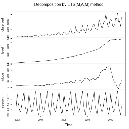
In the model output from the ETS Tool four different decomposition graphs display:
Observed: The actual data
Level: Baseline of data without seasonality
Slope: Rate of change associated with the level
Seasonality: Cyclical effects due to time of year
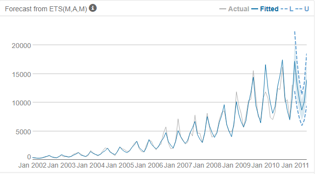
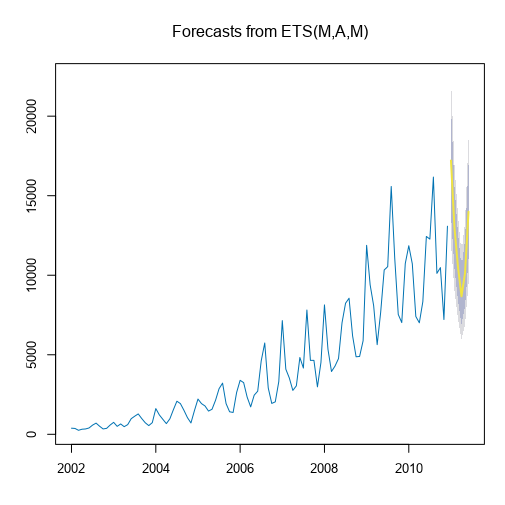
Example forecasts from the ETS model
These graphs shows historical data and future forecasts within a 90% and 95% confidence interval. You can highlight an area of the forecasted plot to zoom into that area.
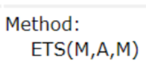
Here is an example method from the report output (R anchor). It has multiplicative error terms, additive trend terms, and multiplicative seasonality terms.
A = additive
M = multiplicative
N = none
In-Sample Error Measures
Lower errors show a better model.
ME: Mean Error is the average difference of actual and forecasted values.
RMSE: Root Mean Square Error is the standard deviation for the differences between forecasted values and actual values.
MAE: Mean Absolute Error is the average sum of the difference from actual to forecasted values.
MPE: Mean Percent Error is the average percent difference between actual and forecasted values.
MAPE: Mean Absolute Percent Error is expressed in a percentage that is useful for reporting.
MASE: Mean Absolute Scaled Error is the mean absolute error of the model divided by the the mean absolute value of the first difference of the series.
Scale-dependent errors are only for use with a single time series scale, and cannot be used with other comparisons on a different scale. This includes the measures ME, MPE, MAE, and RMSE.
Percentage Errors are scale-independent and can be used for comparing forecast between different time series data sets, for example MAPE. Scale-free errors are also scale-independent such as MASE.

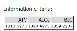
Information Criteria
Lowest values show the best fit.
AIC: Akaike Info. Criterion This measure shows the comparative quality of a statistical model. It balances the goodness of fit with the complexity of the model. AIC is used for comparison of models produced from the same data. AIC cannot show that all models are too inaccurate. It only provides a comparison of the accuracy between the models.
AICc: Akaike Info. Criterion Corrected If the auto option (default configuration) is selected, then the AICc is used if there are 48 or fewer observations
BIC: Bayesian Info. Criterion
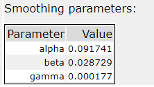
Smoothing Parameters
Alpha: Shows percent of forecasts that are based on the most recent observations. It represents the level of the data.
Beta: Parameter for exponential decay. Usually between 0 and 1. The closer to 1 the higher the weight on more recent observations. It represents the trend of the data.
Gamma: The higher the gamma, the more weight is placed on more recent observations. It represents seasonality of the data. Seasonality increases in proportion to level.
Small values of beta and gamma result in very small changes over time for slope and seasonality.
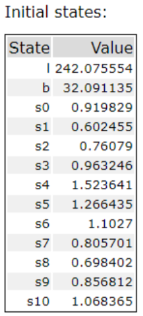
Initial States
Estimates used to calculate AIC.
Which model is the best, ARIMA or ETS? Try both and use the TS Compare tool. It selects the model with the best AIC or AICc score.
For information on how to use the ARIMA tool, please see: https://community.alteryx.com/t5/Alteryx-Designer-Knowledge-Base/How-to-use-the-ARIMA-tool/ta-p/5496....
Forecast
Based on the validation testing, use the best model in the TS Forecast tool. Before using this tool, add the validation sample back to the data set. Note: you can highlight an area of a forecasted plot in the TS Forecast tool to zoom into that area.
A residual is a difference between the observed value and the forecasted value. Good forecasting shows uncorrelated residuals. Residuals should be close to a 0 mean. Otherwise, the forecasts will be inaccurate. If needed, add the mean to all of the forecasts to correct this issue.
After installing the Predictive Tools, Sample Time Series workflows are available in Help, Sample Workflows, Predictive tool samples menu. There are help pages for the Time Series tools, as well as recorded training sessions. Also, there is a free Time Series Forecasting course on the alteryx.com Resources page. Please see the links below.
Credit and thanks goes to Bhumika Patel for the idea to write the article and much of the content.
Additional Resources
https://help.alteryx.com/current/designer/time-series
https://community.alteryx.com/t5/Videos/Time-Series-Analysis/td-p/114070
https://community.alteryx.com/t5/Videos/Time-Series-Modeling/td-p/256421
https://www.alteryx.com/resources/resource-library/predictive-training
An ETS model, otherwise known as exponential smoothing, estimates single variable forecasts using weighted averages of past observations. There is more weight given to recent observations with a gradual and constant rate of decrease for the observation weight over time. Depending on the method used, there is a smoothing equation for one or more of the following: level, trend, and seasonality.
Procedure
Start with a Time Series Decomposition Plot from the TS Plot Tool
Use the TS Plot Tool first to determine what options are best in the ETS Tool with the data. Start with the decomposition plot to investigate the seasonality, trend, and error (remainder) terms of a time series. The TS Plot Tool provides the following plots: Time Series, Season, Decomposition, Autocorrelation, and Partial Autocorrelation. For more information, please see https://help.alteryx.com/current/designer/ts-plot-tool.
Determine the method needed for the ETS terms
The E, T, and S terms represent Error, Trend, and Seasonality. The ETS terms will have the letter of the method used.
A = additive
M = multiplicative
N = none
For example, the model ETS(A,M,N) uses an additive method for the error term, a multiplicative method for the trend, and none for the seasonality.
Typically, the additive method is for trend and seasonal variation that remains mostly constant over time (linear). This method adds the difference in prior observations to predict future values.
Multiplication of the terms is best when the trend and seasonal variation increases or decreases exponentially. The method multiplies previous observations by a factor to determine future values.
Over forecasting of results due to a predicted constant future trend can be prevented using a trend damping method. After using trend dampening, you can compare the forecasting errors between the dampened version and the original to determine which one is more accurate.
Build and validate the ETS model
Commonly, 10 - 30% of the data is used for a holdout validation sample in predictive modeling. This sample is usually the most recent data. It should include at least the number of periods you are forecasting. Validate with the TS Compare Tool using the ETS tool’s Object output and the remaining data.
When the Auto option is selected on the Model Type tab, the ETS tool automatically chooses the best model terms based on the AIC score. When comparing a custom model to auto selections, if the AIC scores are similar, and compare the calculated errors to see what is best.
In the model output from the ETS Tool four different decomposition graphs display:
Observed: The actual data
Level: Baseline of data without seasonality
Slope: Rate of change associated with the level
Seasonality: Cyclical effects due to time of year

Example forecasts from the ETS model
These graphs shows historical data and future forecasts within a 90% and 95% confidence interval. You can highlight an area of the forecasted plot to zoom into that area.


Here is an example method from the report output (R anchor). It has multiplicative error terms, additive trend terms, and multiplicative seasonality terms.
A = additive
M = multiplicative
N = none

In-Sample Error Measures
Lower errors show a better model.
ME: Mean Error is the average difference of actual and forecasted values.
RMSE: Root Mean Square Error is the standard deviation for the differences between forecasted values and actual values.
MAE: Mean Absolute Error is the average sum of the difference from actual to forecasted values.
MPE: Mean Percent Error is the average percent difference between actual and forecasted values.
MAPE: Mean Absolute Percent Error is expressed in a percentage that is useful for reporting.
MASE: Mean Absolute Scaled Error is the mean absolute error of the model divided by the the mean absolute value of the first difference of the series.
Scale-dependent errors are only for use with a single time series scale, and cannot be used with other comparisons on a different scale. This includes the measures ME, MPE, MAE, and RMSE.
Percentage Errors are scale-independent and can be used for comparing forecast between different time series data sets, for example MAPE. Scale-free errors are also scale-independent such as MASE.

Information Criteria
Lowest values show the best fit.
AIC: Akaike Info. Criterion This measure shows the comparative quality of a statistical model. It balances the goodness of fit with the complexity of the model. AIC is used for comparison of models produced from the same data. AIC cannot show that all models are too inaccurate. It only provides a comparison of the accuracy between the models.
AICc: Akaike Info. Criterion Corrected If the auto option (default configuration) is selected, then the AICc is used if there are 48 or fewer observations
BIC: Bayesian Info. Criterion

Smoothing Parameters
Alpha: Shows percent of forecasts that are based on the most recent observations. It represents the level of the data.
Beta: Parameter for exponential decay. Usually between 0 and 1. The closer to 1 the higher the weight on more recent observations. It represents the trend of the data.
Gamma: The higher the gamma, the more weight is placed on more recent observations. It represents seasonality of the data. Seasonality increases in proportion to level.
Small values of beta and gamma result in very small changes over time for slope and seasonality.

Initial States
Estimates used to calculate AIC.

Which model is the best, ARIMA or ETS? Try both and use the TS Compare tool. It selects the model with the best AIC or AICc score.
For information on how to use the ARIMA tool, please see: https://community.alteryx.com/t5/Alteryx-Designer-Knowledge-Base/How-to-use-the-ARIMA-tool/ta-p/5496....
Forecast
Based on the validation testing, use the best model in the TS Forecast tool. Before using this tool, add the validation sample back to the data set. Note: you can highlight an area of a forecasted plot in the TS Forecast tool to zoom into that area.
A residual is a difference between the observed value and the forecasted value. Good forecasting shows uncorrelated residuals. Residuals should be close to a 0 mean. Otherwise, the forecasts will be inaccurate. If needed, add the mean to all of the forecasts to correct this issue.
After installing the Predictive Tools, Sample Time Series workflows are available in Help, Sample Workflows, Predictive tool samples menu. There are help pages for the Time Series tools, as well as recorded training sessions. Also, there is a free Time Series Forecasting course on the alteryx.com Resources page. Please see the links below.
Credit and thanks goes to Bhumika Patel for the idea to write the article and much of the content.
Additional Resources
https://help.alteryx.com/current/designer/time-series
https://community.alteryx.com/t5/Videos/Time-Series-Analysis/td-p/114070
https://community.alteryx.com/t5/Videos/Time-Series-Modeling/td-p/256421
https://www.alteryx.com/resources/resource-library/predictive-training
Labels:
Labels
-
2018.3
17 -
2018.4
13 -
2019.1
18 -
2019.2
7 -
2019.3
9 -
2019.4
13 -
2020.1
22 -
2020.2
30 -
2020.3
29 -
2020.4
35 -
2021.2
52 -
2021.3
25 -
2021.4
38 -
2022.1
33 -
Alteryx Designer
9 -
Alteryx Gallery
1 -
Alteryx Server
3 -
API
29 -
Apps
40 -
AWS
11 -
Computer Vision
6 -
Configuration
108 -
Connector
136 -
Connectors
1 -
Data Investigation
14 -
Database Connection
196 -
Date Time
30 -
Designer
204 -
Desktop Automation
22 -
Developer
72 -
Documentation
27 -
Dynamic Processing
31 -
Dynamics CRM
5 -
Error
267 -
Excel
52 -
Expression
40 -
FIPS Designer
1 -
FIPS Licensing
1 -
FIPS Supportability
1 -
FTP
4 -
Fuzzy Match
6 -
Gallery Data Connections
5 -
Google
20 -
In-DB
71 -
Input
185 -
Installation
55 -
Interface
25 -
Join
25 -
Licensing
22 -
Logs
4 -
Machine Learning
4 -
Macros
93 -
Oracle
38 -
Output
110 -
Parse
23 -
Power BI
16 -
Predictive
63 -
Preparation
59 -
Prescriptive
6 -
Python
68 -
R
39 -
RegEx
14 -
Reporting
53 -
Run Command
24 -
Salesforce
25 -
Setup & Installation
1 -
Sharepoint
17 -
Spatial
53 -
SQL
48 -
Tableau
25 -
Text Mining
2 -
Tips + Tricks
94 -
Transformation
15 -
Troubleshooting
3 -
Visualytics
1
- « Previous
- Next »