Engine Works

jdunkerley79 · ‎10-26-2020

When I was young and starting to program, one of the first things that fascinated me was generating images with fractals. Given an often simple algorithm, you can create incredible images with very little code. The Mandelbrot set is a one such. As an experiment, and to test out the AMP engine, I wanted to experiment with creating one in Alteryx. As usual, BaseA rules apply!

I thought it would also be interesting for people to see some of the iterations I went through rather than just the end product. This first post is only going to concentrate on the computation of the data for the set, the way I chose to produce the image, rendering as a bitmap file, is one for another day.

Quick Overview of How to Calculate the Mandelbrot Set

The Mandelbrot set starts with a simple equation:

With z₀=0 and c being a complex number. This means that z₁=c.

Expanding this into real and imaginary parts:

Let where i is the square root of -1

To produce the picture of the Mandelbrot set, you scan through different values of c and see if the iterative equations tend to infinity or remain bounded. This is normally tested by if the absolute value of z exceeds 2 within a certain number of iterations. The absolute of z_n is:

To speed up the computation slightly, I chose to check when the absolute of z squared exceeded 4.

The colour of the point at c can be produced by how fast the iteration exceeded the limit. I chose to use a colour scheme from D3 - specifically the Rainbow one.

Computing the Iterative Equation in Alteryx

So there a few options of how to create the set within Alteryx. Let's start with the simple part - creating the grid of points we will evaluate across.

The input I chose for this was:

Dim	Min	Max	Points
Real	-2	1	800
Imaginary	-1.1	1	600

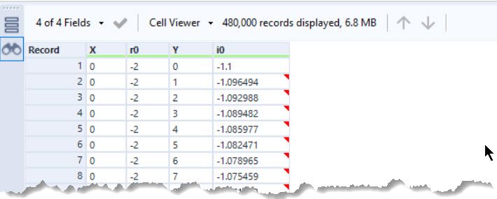
Using a formula tool, can compute the step size (([Max]-[Min]) / (Points - 1)). Feeding this into a generate row tools to make the 800 real points and 600 imaginary points. After this, using an Append Fields tool, which is set to allow all appends, it creates the complete grid of points.

The complication for the iterative equation is that we need to iterate 2 variables and track the numbers of steps. I tried a few different approaches to this.

Approach 1: Iterative Macro

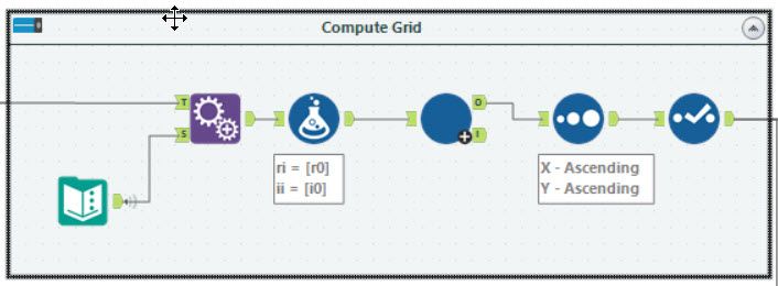
Probably the most obvious is to use an iterative macro. These can be sluggish, but as each iteration will act on the entire grid and a maximum of about 80 steps will be needed, it's not too slow and a straightforward approach. First, let's add a couple of columns to the grid:

Thres: The threshold to declare it is tending to infinity
MaxSteps: Number of steps to test the data on
ri: Current real value
ii: Current imaginary value

Each iteration of the macro does the following:

Compute di the current value of the |z|
Compute the new values for ri and ii
Split the data set looking at those points which have di > thres or if the number of maximum iterations has been reached.
Return those rows to the outer workflow, loop the others with the updated ri and ii values.

This approach was pretty easy and produced a 1080p image in about 45 seconds on my laptop. In this approach, the difference between AMP engine came out slightly slower than the old E1 engine - 52.3 seconds vs 41.1 seconds.

Approach 2: String States

One approach to iterate a value in Alteryx is to use the Generate Rows tool. This is pretty straight forward to iterate a single value, for example, to create 100 rows you can count from 1 to 100. In this case, we need to iterate 3 values - iteration number, real and imaginary values. One simple trick to do this is to keep it as a string:

<Count> <Real> <Imaginary>

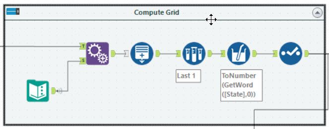
Alteryx provides a handy function GetWord, which allows you to extract a single word from the text. Combining this with the ToNumber and ToString functions, you can construct the iteration:

The Generate Rows tool is set to create a new V_String(48) field. It is initially set to 1 0 0. The step is given by:

ToString(ToNumber(GetWord([State], 0)) + 1) + " "
+ 
ToString(
Pow(ToNumber(GetWord([State], 1)),2) - Pow(ToNumber(GetWord([State], 2)),2) + [r0]
) + " "
+ 
ToString(2 * ToNumber(GetWord([State], 1)) * ToNumber(GetWord([State], 2)) + [i0])

The expression breaks into three parts:

ToString(ToNumber(GetWord([State], 0)) + 1) increments the first value by 1.
ToString( Pow(ToNumber(GetWord([State], 1)),2) - Pow(ToNumber(GetWord([State], 2)),2) + [r0] ) implements the Real part calculation = ToString(2 * ToNumber(GetWord([State], 1)) * ToNumber(GetWord([State], 2)) + [i0]) implements the Imaginary part.

The ToNumber(GetWord([State], 1)) allows you to extract one of the values from the string and convert it back to a number.

The final part of the Generate Rows is the termination condition:

ToNumber(GetWord([State], 0)) <= [MaxSteps]
AND
Pow(ToNumber(GetWord([State], 1)),2) + Pow(ToNumber(GetWord([State], 2)),2) < [Thres]

In this case, the first line checks the number of steps executed. The second evaluates if the iteration has broken out.

After this, a Sample tool is used to pick the final row of each iteration, and then a formula tool extracts the initial number.

Producing a 1080p image with this workflow is substantially slower than the iterative macro approach. Using E1, it took about 8 minutes. AMP gave it a nice performance boost up to about 5 minutes 30 seconds. But with either engine a chunk slower than the first approach.

Approach 3: Spatial Objects

My next approach was to use spatial objects and formulas in the Generate Rows tool. This approach was to use the latitude and longitude of points as real and imaginary values. Each step would add a new point to the current spatial object and then assess when to terminate based on its distance from 0,0 and now many points there are.

Unfortunately, this was a failed experiment as it was much slower than either of the above approaches, so I didn't complete it. I tried generating 80 rows each time and using multi-row formulas but again to no significant success.

The one shout out from this approach is the Spatial Functions. They are often overlooked but provide a lot of power in formula tools when working with spatial objects.

Approach 4: Dynamic Formula

My last approach was to use a dynamic formula to build the iteration in a single formula tool. Starting by defining ri and ii as the current real and imaginary values and initialising them to 0. Additionally, define i to be the step of the iteration. The one catch is I need to know when the iteration terminates - I chose to indicate this by switching i to be a negative value. The following three expressions evaluate one step of the iteration in a formula tool:

i: iif([i]<0,[i],iif([i]>=[MaxSteps] OR [ri]*[ri]+[ii]*[ii]>[Thres],-[i],[i]+1))
t: iif([i]<0,0,[ri]*[ii])
ri: iif([i]<0,[ri],[ri]*[ri]-[ii]*[ii]+[r0])
ii: iif([i]<0,[ii],2*[t]+[i0])

Note, t is needed as ri is mutated before computing ii.

The next step is to extract the XML for these expressions:

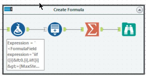
    <FormulaField expression="iif([i]&lt;0,[i],iif([i]&gt;=[MaxSteps] OR [ri]*[ri]+[ii]*[ii]&gt;[Thres],-[i],[i]+1))" field="i" />
    <FormulaField expression="iif([i]&lt;0,0,[ri]*[ii])" field="t" size="8" type="Double" />
    <FormulaField expression="iif([i]&lt;0,[ri],[ri]*[ri]-[ii]*[ii]+[r0])" field="ri" />
    <FormulaField expression="iif([i]&lt;0,[ii],2*[t]+[i0])" field="ii" />

The XML can be found by going to the XML tab in the properties pane for the Formula tool. Using a formula tool to create a copy of this XML, and then a Generate Rows tool to repeat it the maximum steps times. This can then be fed into a Summarize tool in concatenate mode to build a big block of XML.

For initial testing, manually edit the XML to be this long new expression between the FormulaFields tags. If all is working, using a simple batch macro to update a formula tool allows this to be more automated:

The control panel is fed into the formula tool and using an Action tool to update the inner XML between the FormulaFields. The very last thing to remember is i will be the negative value at the end so and additional formula tool is needed to switch signs.

Using my same test of producing a 1080p image, the difference between AMP and e1 was minor (1:06 vs 1:10). I also tested without the batch macro, and this made next to no difference.

Assigning Colours and Rendering the Output

The next step for producing the image is to convert the number of steps taken into a colour.

Starting with a list of colours from the D3 page expressed as hexadecimal strings, add a RecordID. Then using a MOD function, you can filter out, so only the right number of distinct colours is kept. Adding a new RecordID which can then be used with a Find and Replace to join to the computed set. Using Find and Replace avoids the larger data set being sorted but does mean that the record ID needs to be cast as a string using a Select tool.

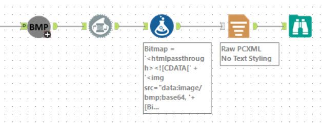
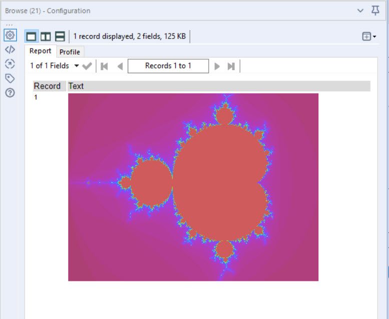
I'm not covering the rendering of a bitmap in this post (hopefully will detail that in a later post) but using a little trickery with blobs and base64 encoding it is possible to render it in a reporting tool. The final output looks like this:

Wrapping Up

Hopefully, this post gives you some insight from the different ways I tried to produce the image. The workflows for this post available below: