Data Science
Machine learning & data science for beginners and experts alike.- Community
- :
- Community
- :
- Learn
- :
- Blogs
- :
- Data Science
- :
- Survival Analysis, Part 3: Using Alteryx
- Subscribe to RSS Feed
- Mark as New
- Mark as Read
- Bookmark
- Subscribe
- Printer Friendly Page
- Notify Moderator
Survival Analysis, Part 1: Introduction
Survival Analysis, Part 2: Key Models
Survival Analysis, Part 3: Using Alteryx (You are here)
In this example, we’ll walk through a use case that looks at applying survival analysis to understand customer churn. Specifically, we will use the R-based Survival Analysis Tool to plot the KM survival curve and determine if different gender groups display different churn behavior. We will also investigate what is the effect of covariates such as gender and monthly bill amount on churn.
You can download the relevant tools from the Alteryx Analytics Gallery if you haven’t done so already.
The tools you will need are:
The Survival Analysis Tool:
The Survival Score Tool:
Data Preparation
Survival analysis assumes that your dataset is set up so that each row represents one person or observation in the overall population. In order to conduct survival analysis, your dataset must include at least the following information as columns:
- A unique ID field (e.g. customer ID), so you can correctly map the predictions back to your data.
- A duration field (such as a customer’s tenure) up to the observation period or the event period, whichever is earlier.
- As an alternative, you could have one column that contains the start date and a second column that contains the event date, but I find that it is usually easier to just work with the duration.
- A censor label if your data is censored (e.g. whether a customer experienced an event or is right-censored). Use 1 to signify that the event (death, attrition, failure, etc.) happened, and 0 to signify that the data is right censored for the individual/observation.
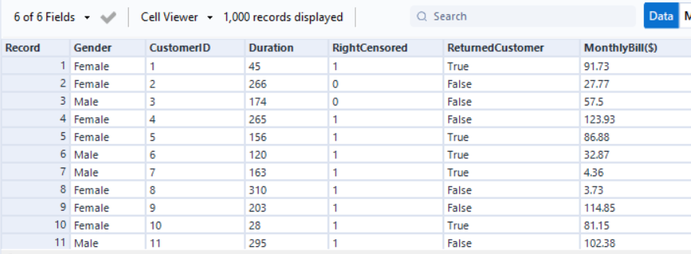
I’ve prepared a mock dataset, and It contains an ID field, a Duration field, a Censor Label field, and three covariate fields, Gender, ReturnedCustomer label, and MonthlyBill($).
To enable a richer analysis of the effect of other covariate/confounding fields on churn, your data could also include columns such as:
- group, gender, income, spending, payment method etc.
The Kaplan-Meier Model in Alteryx
Alteryx has really made it straightforward to construct the Kaplan-Meier model. We simply need to set up a few configurations, so let me walk you through how it is done.
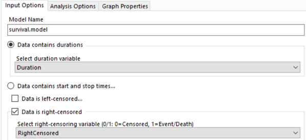
Within the Configuration window of the Survival Analysis Tool, you will find three tabs: Input Options, Analysis Options, and Graph Properties. The first two tabs will impact the outcomes of our model, while the Graph Properties tab is solely concerned with the dimensions and resolution of the graphs.
Input Options:
- Model Name: Give your model a sensible name. Note the name should not contain special characters other than “.” or “_”, and no spaces are allowed.
- Data contains durations / Data contains start and stop times: Select one of these radio buttons based on whether your data contains durations or actual start and stop times. For our sample dataset, the correct choice is “Data contains durations.”
- Data is left-censored / Data is right-censored: These are optional checkboxes, check them only if your data is censored. Since our data is right-censored, meaning that some subjects were lost to follow-up before the event occurred, we will check the appropriate box.
- When checked, you will then need to select the field that corresponds to the censorship label. Double-check that you’ve correctly labeled the censorship; 0 is Censored, and 1 should be the event.
Analysis Options:
- Make sure the Kaplan-Meier Estimate’s radio button is selected.
- You can also select the corresponding check box or boxes to suit your analytical needs.
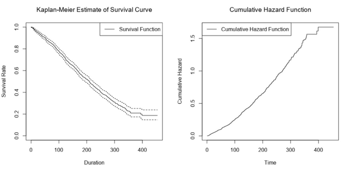
In general, it can be useful to include a confidence interval with your statistical estimates. We can see below that on average, after 200 days, we can expect around 50% of customers to remain with us, or between 45% to 55% retention according to the 95% confidence interval.
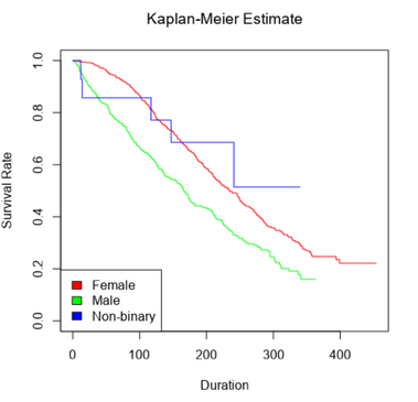
Often, we may want to group by a field to compare how the survival curve varies across groups, and the Survival Analysis Tool has an option that makes it easy for you to do just that! When the "group by" field is used, separate KM curves will be created for each of the groups in the "group by" field.
Pro Tip: When using the Select grouping variable option, make sure the field you select is the first field (column) in the dataset, otherwise Alteryx may throw an error.
As we can see, at any given time point, female customers have a noticeably higher survival rate than male customers. This suggests that we should potentially focus on attracting female users to our platform, as they tend to be more loyal than male customers.
The jagged survival curve of the non-binary gender simply reflects the fact that this group of customers has a relatively low number of observations – as each customer experiences the event of interest, it represents a higher percentage of each person in that group.
The Cox Proportional Hazards Model in Alteryx
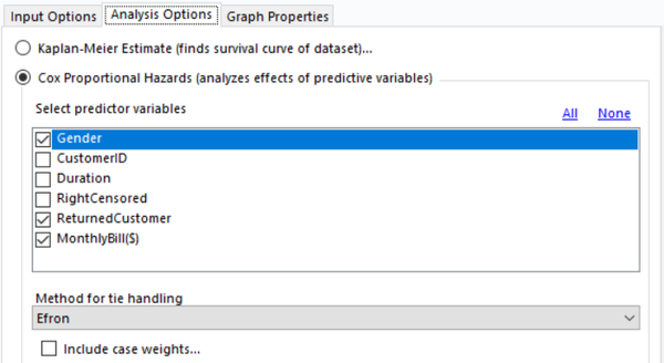
To construct a CPH model in Alteryx, we will continue using the same Survival Analysis Tool. In fact, we can even leave all the configurations in the Input Options to be the same as before. The only part that we need to configure is the Analysis Options.
Analysis Options:
- Make sure the Cox Proportional Hazards option is selected instead of the Kaplan-Meier estimate.
- Select predictor variables: Select the covariate variables that you’d like to incorporate in your survival analysis.
- Method for tie handling: Alteryx provides three methods for dealing with tied times (durations). See the R documentation for more information.
- You can also optionally select a field that contains case weights. Case weights can be used to replicate subjects’ observations, as described in the R documentation.
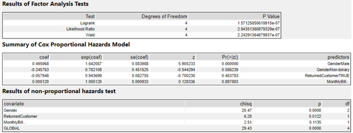
Here is what the results look like:
Note that the Survival Analysis Tool automatically encodes categorical data. In this case, we can see that Gender has been one-hot-encoded (the Gender column doesn’t have to appear at the start of the data to be one-hot-encoded).
- Results of Factor Analysis Tests: This section informs us whether our CPH model is statistically significant. With a p-value much smaller than 0.05, our model is significant here.
- Summary of Cox Proportional Hazards Model: This section is quite similar to linear regression, where we can see:
- the estimated coefficient for each variable (positive means increasing risk, negative means decreasing risk of churn). Like we observed in the KM model, male customers tend to be associated with increased risk (and hence the positive sign here as well).
- The exp(coef) gives us the effect size, it is simply the exponent of the coefficient. The exp(coef) for GenderMale is 1.64, meaning that males increase the churn risk by 64% compared with females. Values near one represent a lower impact on the system.
- The se(coef), z and Pr(>|z|) are used to determine the statistical significance of the variables. We can see that in our model, GenderNon-binary, ReturnedCustomer label, and MonthlyBill are not significantly different from 0, so we can drop these variables. This is in alignment with the exp(coef) values for those features, which show a risk percentage close to 100% or a similar risk level to the comparison feature.
- Results of non-proportional hazards test: This section tests the hypothesis of whether the terms in the model meet the constant proportional hazards assumption. It seems that this assumption is broken by our model since the p-values are small enough to reject the null hypothesis. If the constant proportional hazards assumption is not satisfied, you could consider stratifying the dataset by partitioning it along the time axis, or keep in mind that the effects of covariates may not be linear.
You must be a registered user to add a comment. If you've already registered, sign in. Otherwise, register and sign in.

