 This article is part of the Tool Mastery Series, a compilation of Knowledge Base contributions to introduce diverse working examples for Designer Tools. Here we’lldelve into uses of the Forest Model Tool on our way to mastering the Alteryx Designer:
The Alteryx Forest Model Tool implements a random forest model using functions in the randomForestR package.Random forest modelsare an ensemble learning method that leverages the individual predictive power of decision trees into a more robust model by creating a large number of decision trees (i.e., a "forest") andcombining all of the individual estimates of the trees intoa single model estimate.For more information on how Random Forest Models work, please check out the Community articleSeeing the Forest for the Trees: an Introduction to Random Forestsor the documentation on random forest models by Leo Breiman and Adele Cutler. In this Tool Mastery, we will be reviewing the configuration of the Forest Model Tool, as well as its outputs.
Configuration
There are three tabs in the Forest Model tool's configuration window: Required Parameters, Model Customization, and Graphics Options. Required Parameters is where the basic arguments for training the model are provided to the tool, and is the only required tab.
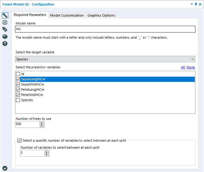
The Model Name argument is where you specify the name given to the Random Forest model you are generating. It can be anything you want, as long as it follows standard R naming conventions: it must start with a letter, and only include letters, numbers, underscores, or periods (dots). Any spaces included in the model name will be replaced with underscores to make the name syntactically valid.
Select the target variable is where you select which field of your dataset you would like to train the model to estimate (predict). Random Forests are essentially an ensemble of decision trees, so they can handle numeric (continuous) or categorical (discrete) target variables. The type of trees constructed to make up the forest will depend on the data type of the target variable. A numeric variable will result in regression trees, where a categorical variable will construct a set of classification trees.
Select the predictor variables is where you specify which variables you would like to use to estimate your target variable.
Number of trees to use is an integer argument, where you tell the model exactly how many trees you want your forest to be comprised of. The default is 500. Generally, a greater number of trees should improve your results; in theory, Random Forests do not overfit to their training data set. However, there are diminishing returns as trees are added to a model, and some research has suggested that overfitting in a Random Forest can occur with noisy datasets.The Report (R) output of the Forest Model tool does include a plot depicting the Percentage Error for Different Number of Trees, which can be used todetermine an appropriate number of trees to include in your model, given your data. If you're not sure where to start, stick with the default value for the number of trees, and then use the plot(s) included in the report output to reduce the number of trees to the lowest value possible while obtaining stable error rates. We will discuss this a little more in the outputs section.
Select a specific number of variables to select between each split is a checkbox option that allows you to choose to specify the number of predictor variables that are randomly sampled as candidates for a split at each split while building out individual decision trees. This random sampling of variables prevents a few strong predictor variables from dominating the splits of all of the individual decision trees. If you leave this option unchecked, the model will determine this value based on an internal rule. For classification forests, the rule is the square root of the number of variables in your data set. For regression forests, the value is the number of variables in your data set divided by three.
The Model Customization tab allows you to perform some additional model tweaking prior to training your random forest model.
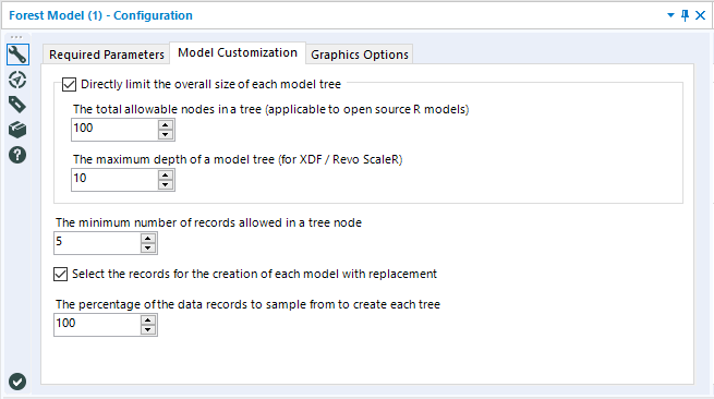
The checkbox option to Directly limit the overall size of each model tree allows you to specify specific limitations on the maximum number of nodes that each individual decision tree in the forest can be comprised of. The two arguments have the same overall functionality, and both are included because there are two different potential packages that this tool can use, depending on if you are working with the standard (open source R) predictive tools installation or the MRCorMMLS version of the predictive tools (used for the in-DB version of the Forest Model Tool).The total allowable nodes in a tree(standard predictive tools) limits thetotal number of nodes that each tree can be comprised of. The maximum depth of a model tree(MRC/MMLS) limits the overall size of a tree by setting a ceiling for the number of levels (of nodes) that can make up a tree
The minimum number of records allowed in a tree node limits the possible smallest size of a terminal node during the training of the individual decision trees that comprise the random forest. The default setting is 5, which means that at least five records from the training data set must "end up" in each terminal node of the tree. Increasing this value will result in an overall reduction of the total nodes in each tree. Both this option and theDirectly limit the overall size of each model tree are ways to manually limit the size of decision trees.
The next two settings are related to what data is used to construct each individual tree.
The Select the records for the creation of each model with replacement option is a checkbox that allows you to specify if the bootstrap samples are sampled with or without replacement. The default is to sample with replacement. Sampling with replacement is a key component of bagging, a meta-algorithm that random forest models are based on, so deselect this option with care.
The percentage of the data records to sample from to create each tree argument allows you to control whether the full training data set, or a random subsample of the data set will be used for creating each bootstrap replicate (i.e., training data sub-sample used to train an individual tree).
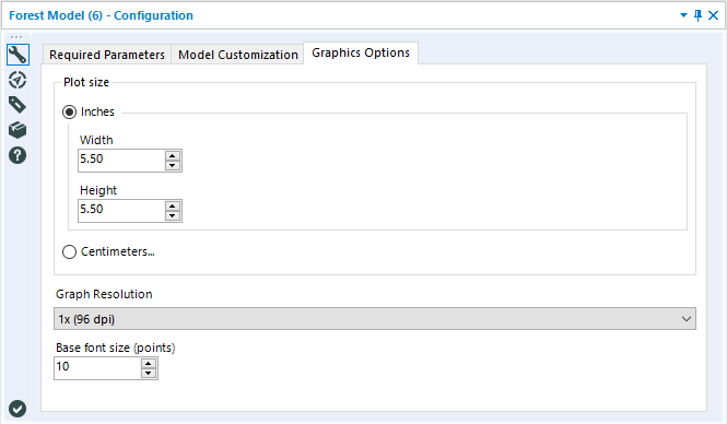
The final tab, Graphics Options, allows you to set the size of the output plots (in Inches or Centimeters) as well as specify the image’s resolution and base font size.
Outputs
There are two output anchors of the Forest Model Tool: the O (Output) anchor and the R (Report) anchor.
The O Anchor includes the model object, which can be used as an input for a few other tools, including the Score Tool if you would like to estimate values for a different dataset using your model, or to the Model Comparison Tool if you’re interested in validation-data based metrics for your model.
The R Anchor is a report on the model that was trained by the Forest Model tool.
The first few rows of the report are mostly a summary of how the model was built based on arguments included in the configuration. The call is the function that was used in the R code to train the model. The arguments specified in the configuration are listed in the next row, as Type of forest:this is either classification or regression, and will directly depend on your target variable,Number of trees: which is specified by the Number of trees to use argument in the first tab, and Number of variables tried at each split: which was either determined by the model, or specifically specified in the configuration (first tab).
The report components following the call and argument is information are used to assess the model. Many of the metrics used to asses Random Forest models are based on OOB, meaning out of bag, measurements. To understand these metrics, it is important to first understand what OOB is.
Random Forest models create many slightly different decision trees by randomly subsampling (with replacement) the training data set, to create a "new" data set for each individual tree. The sampling with replacement causes approximately 1/3 of the original training data to be excluded from training each individual decision tree. This excluded data is referred to as the out-of-bag (OOB) observations. The out of bag data can then be used to create out of bag (OOB) error estimates by running data through each individual tree where it was excluded from training the tree, and then aggregating the results of each tree to a single prediction. The out of bag error can be used in place of cross-validation metrics. Through research,OOB has been proven to be an unbiased measure of performance in many tests and is typically considered to bea conservative measure, biased towards higher percent error values that metrics based on independent validation data.
The specific metrics returned will depend on if you trained a classification or regression forest.
Classification Forests
The OOB estimate of error rate reported in the report table output is the percentage of misclassified records based on the estimate of the trees where the record was excluded from training.
The Confusion Matrix is also based on OOB estimates and compares the OOB estimates (in columns) to the actual classifications (rows). We can see that the Iris-setosa were correctly classified for all records, where Iris-versicolor and Iris-virgninica were more prone to misclassifications.

The next component of a classification forest report is a set of plots. The first plot is of the error rates of the Random Forest model in comparison to the number of trees in the model object.
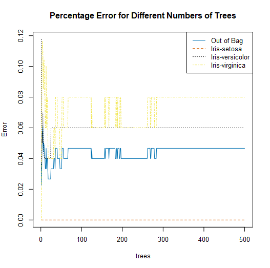
A line for each classification in your target variable is plotted, in addition to a general out of bag line. The out of bag line is the average error rate across all classes.
This plot can be helpful in determining the appropriate number of trees to include in your random forest model. In this plot, we see that error rates stabilize for all classes after about 300 trees, which would indicate that 300 trees would be adequate for estimating your target variable.
The second plot depicts an estimate of predictor variable importance.
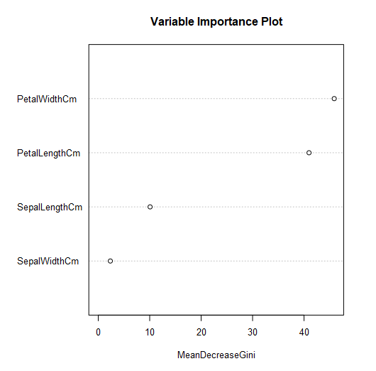
Mean Decrease Gini measures how important a feature (predictor variable) is, by calculating a forest-wide weighted average for how much that predictor variable reduced heterogeneity in a given split. This can be used to help with variable selection. Here, we see that Petal Width and Petal Length were the most important for generating this tree. If you would like more detail, you might find this StackExchange posthelpful.
Regression Forests
The two metrics included in the table are the mean of the squared residuals and the explained variance, both based on OOB estimates of the target variable.

The mean of squared residuals (also known as mean squared error (mse)) is calculated with the OOB estimates of target values in comparison to the known target variable value. The metric itself is the average squared difference between the (OOB) estimated value and the known value. The means of squared residuals should always be a positive number. Values closer to zero suggest a better model.
Explained variance is the fraction of variance in the response that is explained by the model, and is calculated as 1 - the mean square error (mse) divided by the variance of the target variable. Unexplained variance is a result of random behavior (noise) or poor model fit. A higher value for this metric suggests a better model.
There are also two plots included in a report for a regression forest. The first plot is a visualization of the percent error vs. the number of trees in the forest.
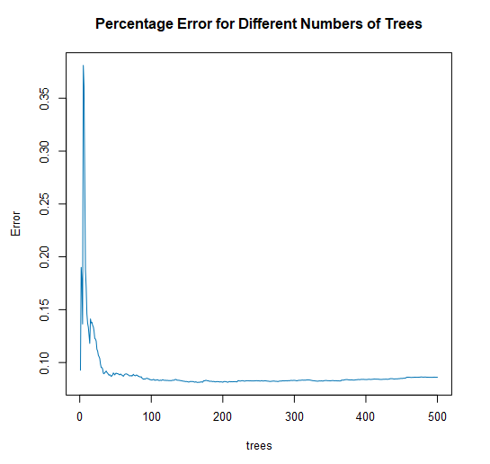
With this plot, you are looking for a point where the error stabilizes, and there is no longer a reduction in error as more trees are added to the forest. This plot can help you refine your model to include fewer trees without losing predictive power.
The second plot is a variable importance plot.
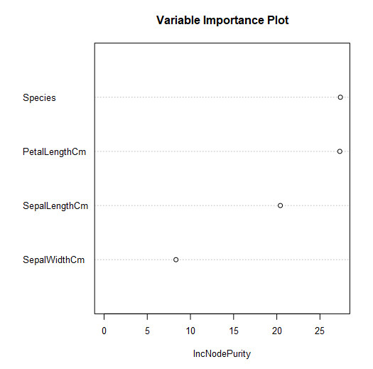
This plot depicts the relative importance of the predictor variables for estimating the target variable, based on the increase in node purity. Increase in node purity relates to the loss function used to determine splits (nodes) in the individual decision trees that make up the forest. For regression trees, this loss function is mean square error (mse). Variables with more predictive power will have higher increases in node purity, resulting in a higher value for IncNodePurity.
By now, you should have expert-level proficiency with the Forest ModelTool! If you can think of a use case we left out, feel free to use the comments section below! Consider yourself a Tool Master already? Let us know atcommunity@alteryx.comif you’d like your creative tool uses to be featured in the Tool Mastery Series.
Stay tuned with our latest posts everyTool Tuesdayby followingAlteryxon Twitter! If you want to master all the Designer tools, considersubscribingfor email notifications.