Data Science
Machine learning & data science for beginners and experts alike.- Community
- :
- Community
- :
- Learn
- :
- Blogs
- :
- Data Science
- :
- Blending Fine Wine with Alteryx: An Optimization T...
- Subscribe to RSS Feed
- Mark as New
- Mark as Read
- Bookmark
- Subscribe
- Printer Friendly Page
- Notify Moderator
The Optimization Tool has been a part of the Alteryx predictive tool suite for a few years now, but there has been a fairly limited discussion of how it works under the hood, the types of problems it can address, and the different ways the tool can be configured and used (exceptions to this are excellent articles by Philip Mannering, SydneyF, and JoeM).
There are actually numerous types of optimization methods. The algorithms supported by the Optimization Tool in Alteryx are linear programming, quadratic programming, and mixed integer linear programming. Last week I explained how linear programming works and discussed the wine blending use case. Today I walk you through how to perform this analysis in Alteryx Designer. I will cover the other two algorithms in later posts.
The Optimization Tool is part of the Prescriptive tool group. To use it, you will need to install the Alteryx Predictive Tools, if you have not done so already.
Click on the Predictive tool group, and drag the Optimization tool onto the canvas. The tool has four possible inputs, all of which are optional, and three outputs. To solve this problem, we will not be using any of the inputs, but will in subsequent posts.
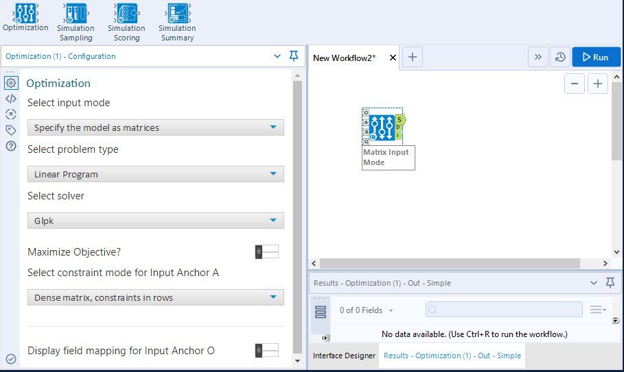
The Configuration panel for the tool is shown in Figure 1. The Select input mode option indicates how the mathematical program will be specified. It defaults to the use of matrices (e.g., standard tables). For larger problems, this is definitely the right choice, and the use of this approach to specify a model will be covered in subsequent posts. However, for this problem, specifying the model using matrices is really overkill since there are only two decision variables and three constraints, so we can take advantage of a more direct method of specifying the model.
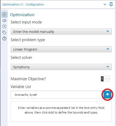
In the Configuration panel, select “Enter the model manually” as the Select input mode option, which will cause the Variable List option to appear. Next, for the Select solver option select “Symphony” as the solver to use. A solver is the software that actually “solves” the linear program. By selecting Symphony, you are actually selecting the relevant solver out of a suite of solvers that have been developed by the COIN-OR project. Based on our experience, the COIN-OR solvers run faster than the default GLPK solver for linear programs. Finally, enter the string “Grenache, Syrah” (without quotes) for the Variable List option. When you are done, your Configuration panel should look like the one shown in Figure 2. To proceed, press the “+” button (circled in red in Figure 2).
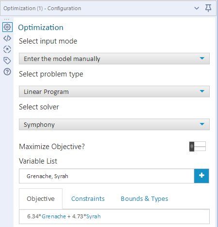
Pressing on the “+” button will cause a new, tabbed, set of options to appear. The first of these options (which is the one shown first) is Objective, where we want to type in the objective function, using standard formula notation, into the provided box, as illustrated in Figure 3.
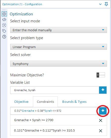
Next, click on the Constraints option tab, where we can enter the three constraints, and is shown in Figure 4. Enter the first constraint in the provided box, and then press the “+” button to add it to the constraint set. This action will also provide you with a box to enter the second constraint. Enter this constraint and the third constraint, pressing the “+” button after each constraint is entered.
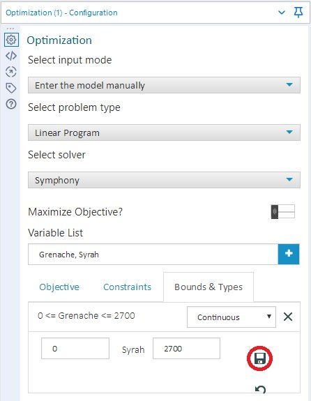
The last step is to enter the Bounds & Types options, as shown in Figure 5. By default, the bounds of the decision variables are set between 0 and infinity. The default lower bounds of 0 is correct for our problem. The default upper bounds could be used without impacting the solution of this linear program (for reasons given in my last post), but we will change them to the correct value of 2700 liters, as shown in the figure, for logical consistency. After changing each upper bound, click on the “disk” icon (circled in red in the figure) to save the change. The default decision variable type is “Continuous” (the other choices are binary and integer), which is appropriate for this application, so no changes are needed with respect to the decision variable types.
Connect a Browse Tool the the “I” output of the Optimization Tool on the canvas and run the workflow. The most complete and user friendly report of the model’s results is given in the interactive report shown in the Browse Tool. The best way to view this report (shown in Figure 6) is to open the contents of the Browse Tool in a new window. The upper left-hand corner of the report provides a summary of the solution, with the critical item being the optimal value of the objective function (the total cost of the wine in a least cost blend), which is the $14,013 we saw in the graphical solution. The upper right-hand corner of the report gives the value of each of the decision variables, indicating that the final blend consists of 1928.57 liters of Syrah and 771.43 liters of Grenache. The lower left-hand corner of the report indicates which constraints are the binding constraints for the solution. A constraint is binding when it has a “slack” value of zero, where slack is defined as the difference between the value of the bound of the constraint and the value of the constraint equation at the optimal solution. Slack values of zero are shaded pink, which corresponds to the cases produced and volatile acid constraints, consistent with our graphical analysis.

Besides the interactive report, the “S” output of the Optimization Tool provides the key elements of the solution (the objective function value and the optimal value for each of the decision variables), which can easily be used as an input to other Alteryx tools downstream. In addition, the “D” output contains all the information contained in the interactive report, but as a name-value pair table. This table can be easily manipulated using the Filter and Text To Columns tools to extract any relevant piece of information about the model solution.
In my next post in the Optimization series, we will look at how to use the tool to create a stock portfolio which minimizes risk for a desired expected return level using quadratic programming, and how to use and create Alteryx tables to specify the quadratic program itself.

Chief Scientist
Dr. Dan Putler is the Chief Scientist at Alteryx, where he is responsible for developing and implementing the product road map for predictive analytics. He has over 30 years of experience in developing predictive analytics models for companies and organizations that cover a large number of industry verticals, ranging from the performing arts to B2B financial services. He is co-author of the book, “Customer and Business Analytics: Applied Data Mining for Business Decision Making Using R”, which is published by Chapman and Hall/CRC Press. Prior to joining Alteryx, Dan was a professor of marketing and marketing research at the University of British Columbia's Sauder School of Business and Purdue University’s Krannert School of Management.
Dr. Dan Putler is the Chief Scientist at Alteryx, where he is responsible for developing and implementing the product road map for predictive analytics. He has over 30 years of experience in developing predictive analytics models for companies and organizations that cover a large number of industry verticals, ranging from the performing arts to B2B financial services. He is co-author of the book, “Customer and Business Analytics: Applied Data Mining for Business Decision Making Using R”, which is published by Chapman and Hall/CRC Press. Prior to joining Alteryx, Dan was a professor of marketing and marketing research at the University of British Columbia's Sauder School of Business and Purdue University’s Krannert School of Management.
You must be a registered user to add a comment. If you've already registered, sign in. Otherwise, register and sign in.
