Data Science
Machine learning & data science for beginners and experts alike.- Community
- :
- Community
- :
- Learn
- :
- Blogs
- :
- Data Science
- :
- Getting to Know Optimization: Linear Programming
- Subscribe to RSS Feed
- Mark as New
- Mark as Read
- Bookmark
- Subscribe
- Printer Friendly Page
- Notify Moderator
Linear programming is the oldest of the mathematical programming algorithms, dating to the late 1930s. The method can either minimize or maximize a linear function of one or more variables subject to a set of inequality constraints. The function to be optimized is known as the objective function, and in many business applications it often involves minimizing cost or maximizing revenue. The areas where linear programming is applied include determining the optimal product mix to maximize revenues, how to best allocate fixed capital equipment and human resources across different activities, optimizing workforce scheduling, blending or mixing raw ingredients to produce a final product at the lowest possible cost, efficiently transporting and storing items, and developing production plans that meet demand at minimal cost. These application areas are common across a wide variety of industry verticals, ranging from airlines to agriculture.
Using Linear Programming to Blend a Fine Wine
The following blending/mixing application is used to illustrate how linear programming works.
Next week's part 2 will describe one method that can be used to set up a linear programming model in the Alteryx Designer Optimization tool to solve this problem. The use case involves a bottler and marketer of wine that wants to produce 300 cases of a Rhone style red wine blend that will be perceived as being of high quality on the part of customers, but at the lowest possible cost.
The two most commonly used grape varieties in Rhone style blends are Grenache and Syrah (also known as Shiraz), both of which are available for purchase on the bulk wine spot market. The company needs to determine the amount of each wine to purchase to create a final product that will be perceived as high quality, at the lowest possible cost.
In this case, the “lowest possible cost” is the objective function of the linear programming problem we will solve, and is simply the sum of the amount of each wine used, multiplied by its cost per unit (price of the wine on the spot market). The amount of each wine to purchase and blend are the variables over which we are optimizing, and are technically known as “decision” or “control” variables. The “perceived as high quality” portion of their goal must be implemented with several model constraints. Without those constraints, the solution to the problem is obvious; purchase enough of the lower-priced of the two bulk wines to create 300 cases of wine. The question becomes, how do we set up the model constraints in a way that will result in a high-quality wine blend?
Creating Quality and Other Constraints
An appropriate way to create the needed quality constraints is to take advantage of sensory data that relates tasters’ perceptions of quality to observable chemical properties of the wine. Research has found that a number of chemical properties of wine are associated with quality perceptions. For illustrative purposes, we will only focus on the two most important ones; alcohol content and volatile acidity. The relationships between chemical properties of wine and quality perceptions are determined using a predictive model. In this case, the Forest Model tool was best able to predict the sensory data. Using this model, the Partial Dependency Tool (located in the Predictive District of the public Alteryx Analytics Gallery) is used to trace the relationship between alcohol content (measured on a percentage volume basis) and perceived quality, and is shown in Figure 1.
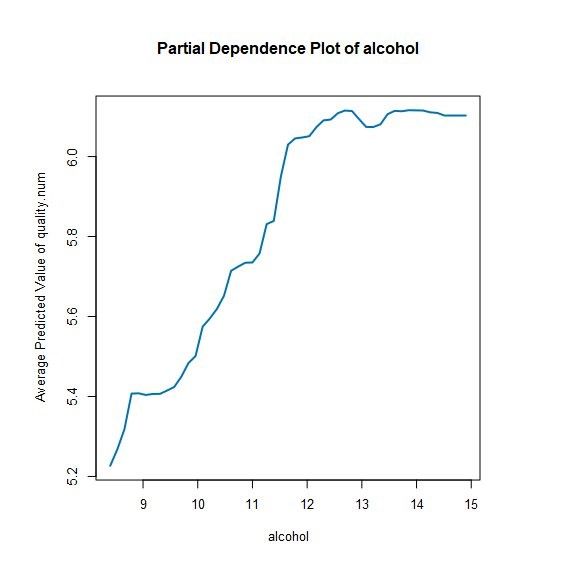
The figure reveals that as the alcohol content of a wine drops below about 11.5% of volume, perceptions of wine quality rapidly decline, while an increasing alcohol content beyond 11.5% has little effect on quality perceptions. Perceptually, alcohol influences mouthfeel (the higher the alcohol content, the heavier and warmer the wine feels in the mouth). Given this, we want to constrain the blend to have an alcohol content that is greater than or equal to 11.5%.
Figure 2 provides a similar plot for volatile acidity. In this case, the figure reveals that as volatile acidity rises above 0.38 grams per liter, perceptions of red wine quality rapidly decrease (high levels of volatile acidity impart a vinegary aroma and taste to wine). As a result, the final blend should have a volatile acidity that is less than or equal to 0.38 grams per liter.

In addition to the perceived quality constraints, another constraint is needed to make sure that 300 cases will be produced. Linear programming requires the use of inequality constraints, when we would like an equality constraint for the number of cases produced. Since we are attempting to minimize cost, we can state that the amount of wine produced needs to be greater than or equal to 300 cases, and the final solution will just meet the quantity constraint (technically, the quantity constraint is said to be “binding”) since a lower total cost can be obtained by reducing the amount of wine used until it equals 300 cases. Finally, a lower bound of zero needs to be placed on the amount of each of the two wines, otherwise, the optimal solution may indicate that a negative amount of one of the wines should be used in the final blend. An upper bound of 300 cases for each wine is also needed since it is expected by the underlying software being used. It turns out, since we are minimizing cost, providing values for the upper bounds above 300 would not change the final solution (the most of either wine that could be used which minimizes cost is 300 cases).
Completing the Linear Program
The relevant characteristics of the two wines are as follows:
- Grenache
- Spot market price: $6.34 per liter
- Alcohol: 13.1% by volume
- Volatile acidity: 0.31 grams/liter
- Syrah (Shiraz)
- Spot market price: $4.73 per liter
- Alcohol: 11.2% by volume
- Volatile acidity: 0.38 grams/liter
The Syrah has a lower price than the Grenache available on the bulk wine spot market, but neither its alcohol content (too low) and volatile acidity (too high) meet the quality constraint. Consequently, a blend of the two different wines will be needed to minimize cost.
At this point we have all the needed information, but, the information needs to be placed in comparable units. The current information is in cases, dollars per liter, grams per liter, and percent by volume. The natural common unit to base things on is liters. A case of wine contains 9 liters, which means that 300 cases is equal to 2700 liters of wine. As indicated above, since we are minimizing cost, exactly 2700 liters of wine will be produced, which allows us to convert the minimum acceptable alcohol content (11.5% by volume) to 310 liters of alcohol (11.5% of 2700 liters), and the maximum allowable volatile acidity of the blend to 972 grams (0.38 multiplied by 2700).
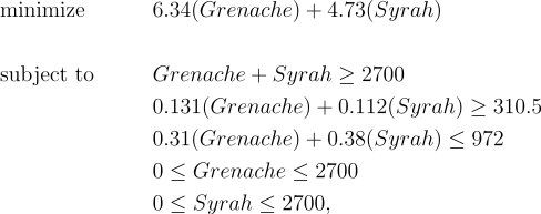
Given all the above, the linear program that needs to be solved is
where Grenache is the number of liters of the Grenache bulk wine to use in the blend, and Syrah is the number of liters of Syrah to use.
How Linear Programming Works
Our wine blending linear program is simple enough that the path to the solution can be shown in a sequence of graphs, which are drawn within the neighborhood of the solution. The axes of the charts are the amounts of each type of wine in the blend. Figure 3 illustrates the effect of the constraint that the final blend contains 11.5% of alcohol or more. The blue line in the lower-left of the figure represents the alcohol constraint. Every point along the line represents a combination of the two wines that results in the final blend having an alcohol content of exactly 11.5%. Any point in a southwesterly direction of the line has less than 11.5% alcohol, so is said to be “infeasible” (since it does not satisfy the alcohol constraint), while points on the line or in a northeasterly direction from the line (which are shaded gray) do meet the constraint, and are said to be “feasible.”
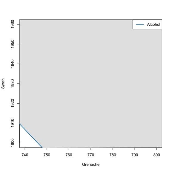
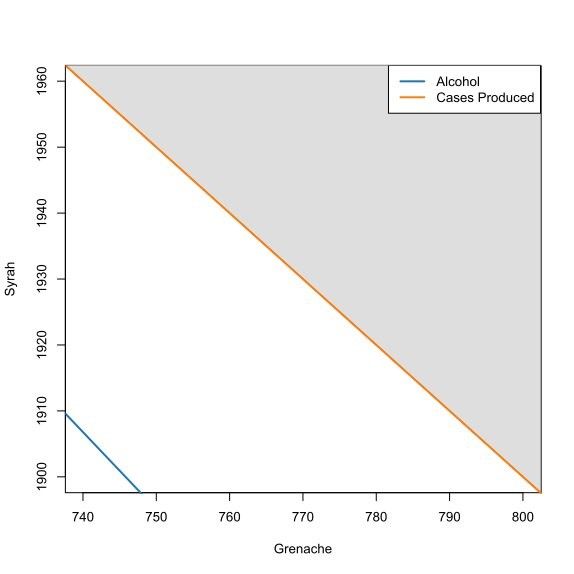
Figure 4 examines the effect of adding the constraint that 300 or more cases need to be produced (the orange line). Every point on the orange line corresponds to the production of exactly 300 cases of wine, while points to the southwest of the line result in fewer than 300 cases being produced, and points to the northeast of the line (shaded gray) represent total cases produced that exceed 300. One thing to notice is that within the neighborhood of the optimal solution, any point that meets the case production constraint also meets the alcohol constraint. Because of this, the alcohol content constraint is said to be “non-binding”, and does not influence the final solution. In addition, this second constraint has reduced the size of the feasible (gray shaded) region.
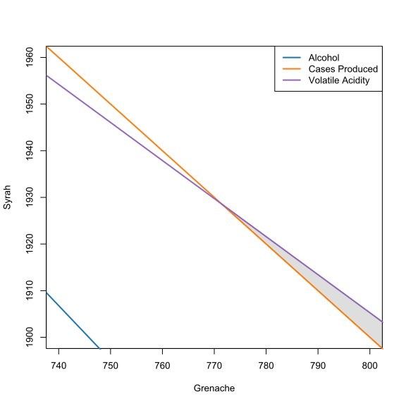
The final constraint that needs to be added is for volatile acidity, which is different from the other two constraints, since it involves a maximum permissible constraint, rather than minimum permissible constraint. As a result, points along this constraint, and points in a southwesterly direction from it meet the constraint, while those in a northeasterly direction do not. Figure 5 shows how the inclusion of this constraint significantly reduces the feasible region of the linear program to a triangular area in the southeast of the plot that starts close to the middle (at the point where the volatile acidity constraint intersects the cases produced constraint). Points between the two constraints that are northwest of their intersection do not meet either of the constraints. Since these two constraints define the feasible region of this linear program, they are called “binding” constraints.
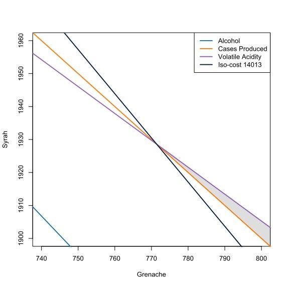
Given the set of constraints, we can find the least cost combination that meets both of the binding constraints by adding the lowest value iso-cost line (the line along which the combination of Syrah and Grenache have the same total cost) to the graph that meets both binding constraints, which is shown in Figure 6. As shown in the figure, the lowest iso-cost line that meets both constraints passes through the intersection point of the two constraints, and corresponds to a total cost of $14,013. Graphically, an iso-cost line of a lower value amounts to a parallel shift of the iso-cost curve to the southwest, however, any shift like this results in an iso-cost line that does not meet the two binding constraints. “Eyeballing” the figure indicates that the least cost blend will contain slightly over 770 liters of Grenache and slightly under 1930 liters of Syrah.
While we can fairly easily solve this linear program graphically, making it even slightly more complex, say by adding another constraint (such as for the total acidity of the wine) or allowing wine from a third grape variety (such as Mourvèdre) to be added to the blend would complicate the analysis, causing the graphical methods to quickly break down. Adding additional constraints adds additional lines to the graph, which is manageable up to a point, but quickly becomes problematic. In contrast, adding another wine to the blend (resulting in a third decision variable) means we need to move from a two-dimensional graphical analysis to a three-dimensional analysis (possible, but challenging), while adding a fourth grape variety would move us to a four-dimensional space (where a graphical approach completely breaks down). Fortunately, the optimization methods used in linear programming are robust to the addition of both more constraints and decision variables.

Chief Scientist
Dr. Dan Putler is the Chief Scientist at Alteryx, where he is responsible for developing and implementing the product road map for predictive analytics. He has over 30 years of experience in developing predictive analytics models for companies and organizations that cover a large number of industry verticals, ranging from the performing arts to B2B financial services. He is co-author of the book, “Customer and Business Analytics: Applied Data Mining for Business Decision Making Using R”, which is published by Chapman and Hall/CRC Press. Prior to joining Alteryx, Dan was a professor of marketing and marketing research at the University of British Columbia's Sauder School of Business and Purdue University’s Krannert School of Management.
Dr. Dan Putler is the Chief Scientist at Alteryx, where he is responsible for developing and implementing the product road map for predictive analytics. He has over 30 years of experience in developing predictive analytics models for companies and organizations that cover a large number of industry verticals, ranging from the performing arts to B2B financial services. He is co-author of the book, “Customer and Business Analytics: Applied Data Mining for Business Decision Making Using R”, which is published by Chapman and Hall/CRC Press. Prior to joining Alteryx, Dan was a professor of marketing and marketing research at the University of British Columbia's Sauder School of Business and Purdue University’s Krannert School of Management.
You must be a registered user to add a comment. If you've already registered, sign in. Otherwise, register and sign in.
