Tool Mastery
Explore a diverse compilation of articles that take an in-depth look at Designer tools.- Community
- :
- Community
- :
- Learn
- :
- Academy
- :
- Tool Mastery
- :
- Tool Mastery | Optimization
Tool Mastery | Optimization
- Subscribe to RSS Feed
- Mark as New
- Mark as Read
- Bookmark
- Subscribe
- Printer Friendly Page
- Notify Moderator
10-12-2018 03:20 PM - edited 08-03-2021 03:34 PM

First added to Alteryx Designer in version 10.6, the Optimization Tool is a member of the PrescriptiveTools (included with the Predictive Tools installation) and allows you to solve optimization problems. MathematicalOptimization is the selection of the best possible option(s), given a set of alternatives and a selection criterion.
Optimization is used for a wide variety of applications across many differentindustries. One general example of a problem that can be solved with optimization is the Knapsack Problem, where given a collection of items (each with a weight and value) determine which combination of items to take in your knapsack, maximizing value without going over the maximum weight you are able to carry.
There are three programming models availableto you in the Alteryx Optimization Tool;Linear Programming,Mixed Integer Programming, andQuadraticProgramming.
Linear programming is best for solving questions like "What mixture of ingredients should I use for plant fertilizer?", based on plant needs, available components, cost, etc, or "How much should we charge for each seat on a flight to London?" based on customer demand. Constraints and variables in a linear program should be continuous, meaning that they can take on any positive numeric value.
Mixed Integer programming is best when some (but not necessarily all) variables are restricted to integer values. This is different from linear programming, where variables can take on any continuous value. Examples of Mixed integer problems include assigningairline crews to cover everyleg of a flight while minimizing cost, and meeting restrictions like minimum rest times, or how many units of raw material to purchase, based on cost and anticipated production. For a verbose example of mixed integer programming in medicine, please see this article from J. Cole Smith and Z. Caner Taskin.
Quadratic programming allows for the optimization of a quadratic objective function, and is one of the simplest forms of non-linear programming. Examples of Quadratic programming problems include portfolio optimization. For additional information on quadratic programming, please see this Wiki Page from Northwestern, or this example in Alteryx, posted on the Community.
The Optimization Tool in Alteryx is very powerful, but it can feel intimidating and tricky to configure. Part of this might be because it seemingly has more input anchors than any other Tool in Designer.
Just for now, let's not worry about the inputs. We will tackle them a little later. Before jumping into any of the configurations the first step for using the Optimization Tool is to think about the question you are asking, and what you expect as a solution. This will help you determine if the Optimization is the right tool for your use case, and guide how you set up your problem.
A few example questions to think about are; What are your constraints? What would you like to be “optimized” (i.e., maximized or minimized)? What rules must be met in your solution? What type of result are you expecting to see as a solution?Taking time to answer these questions and think through your problem before you start fussing with the Tool's configuration will make your life much easier. I promise.
Once you have an idea of what and how you would like to optimize, youcan then determine which programming model you would like to use (Linear, Mixed Integer, or Quadratic) and get down into the inputs.
Inputs
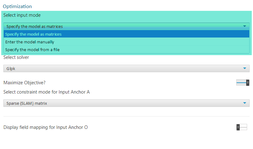
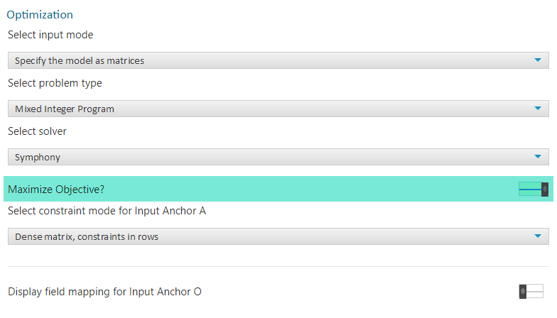
There are three options for input modes. You can enter the model as a series of matrices, enter the model manually (using mathematical notation), or specify the model from a file.
Specify the Model as Matrices
When you elect to use the matrix input mode the input anchors O and A are required, but B and Q are optional.
In this Tool Mastery, each input will be demonstrated for the same Mixed Integer Program. For context, in this example we are attempting to optimize the products we stock in a grocery store. We would like to stock one product in each category (Peanut Butter, Jam, Bread, and Milk), maximizing profit while not exceeding the space available on our shelves.
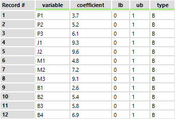
The O anchor is where you provide the decision variables (the options you are selecting from), their coefficients in the objective function (how one option is selected over another), and (optionally) their bounds and types.
Here, we have our options for products. The variable column is the name of each product, the coefficient is what will be optimized (maximized or minimized), and in this use case is the profit for each product. lb, ub, and type are the lower bound, upper bound and variable type, respectively. These three fields are optional but set the minimum and maximum possible values for each option to take on, and the variable type. The variable type can be set to "B" for binary, "C" for continuous, or "I" for integer. The default for variable type is continuous. The variable type will impact how the optimization treats possible solutions with these variables.
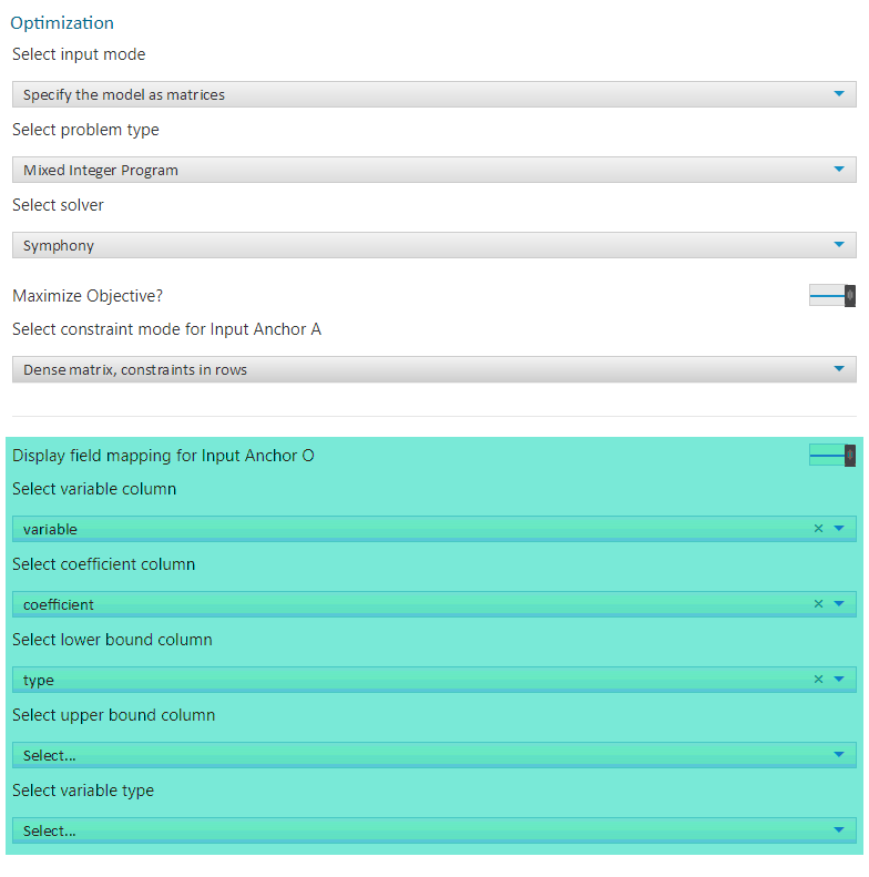
Starting with version 11.0, there is an option to map the fields for Input Anchor O.This allows for more flexibility in field names if you do not feel like following the canonical naming convention.
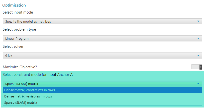
The A anchor is the input for the constraint matrix. You have three options for how the matrix is organized; a Dense matrix with your constraints in rows, a Dense matrix with your variables in rows, or a Sparse (SLAM) matrix.
Dense Matrix, Constraints in Rows
In this format, each row in your input matrix corresponds to a constraint.
In this case, the first row is the size of each product, and the following rows are binary, indicating the type (Peanut Butter, Jam, Milk, Bread) of each product (0 = false, 1 = true)
Dense Matrix, Variables in Rows
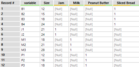
In this format, the variables are now in each row, and the constraints are in columns.
The first column is the size of each object and the following columns indicate which product type each individual product belongs to. Nulls indicate the product is not a member of the given product type, and 1s indicate that the product is a member of the group.
SLAM Sparse Matrix
The SLAM sparse matrix is an input type whereall of the Null's or 0's seen in the previous two matrix configurations are removed. SLAMrefers to an R package that can effectively "translate" sparse matrices when they are provided in the correct (SLAM) format. Using a sparse matrix input can help for optimization problems withlarger constraint sets because sparse matrices take up considerably less memory than their dense counterparts.
A SLAM matrix consists of three required fields; i, j, and v. the i field is a row index, and the j field is a column index. Together, the i and j fields act as matrix coordinates, letting the interpreter know where in the original matrix a given value occurred. The v field is the non-zero value of the matrix cell. If the coordinates of a matrix cell are missing from a sparse matrix, it is assumed that the value for that cell is equal to zero.
Sparse matrix mode always assumes constraints in rows.
In our grocery stocking example, the first row of the sparse matrix is 1, 1, 12. This is because inthe dense matrix form (constraints in rows), the first row of the firstcolumn was equal to 12. The second row, 2, 1, 1, gives the value of the second row of the first column.This pattern continues for each cell in the constraints in rows matrix, skipping cells where the value is 0.
For help converting your data into a sparse matrix, please see the example included in the attached workflow.
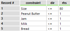
The B anchoris used to provide direction (less than, greater than, or equal to for constraint values) for the variables, and becomes required when this information is not provided in the A anchor input (as is the case in our current example, for details on including dir and rhs in anchor A, please see the help documentation). The columns of the B input are the constraint (the names should match the names provided in input anchor A), the direction, abbreviated as dir, and the right-hand side of the equation, a numeric value (abbreviated as rhs).
This input states that the total size of all selected items must be less than or equal to 80 and that the total number of selected items from each category must be less than or equal to 1.
The (optional) Q anchor only comes in to play when you are specifying a quadratic program in matrix mode. It is where you provide the quadratic portion of the objective function, and can be specified as a dense or sparse matrix. If you are specifying it as a dense matrix, the field names should correspond to the decision value names that were defined in your O anchor. If you are specifying it as a sparse matrix, it should follow the SLAM matrix format with column names i, j, and v. For an example of this input (as a dense matrix), please seethis Designer Discussion Thread.
Enter the model manually
This is an interactive interface, where you can specify the objectives and constraints directly as an equation. This type of model specification does not require any connections made to the input anchors.I won't get too deep into configuring this type of input, because there is an excellent article on Community calledOptimization Tool: Entering a Model Manuallythat demonstrates this configuration step by step, but I will demonstrate what the equations will look like. For the grocery stocking question we've been working with, the equation looks like this:
3.7*P1 + 5.2*P2 + 6.1P3 + 9.3J1 + 9.6J2 + 4.8M1 + 7.2M2 + 9.1M3 + 2.6B1 + 5.4B2 + 5.8B3 + 6.9B4
Where the coefficient for each variable is the profit, andthe value that will be maximized (or minimized, depending on how the optimization problem was set up). You would specify this in the Objective Tab.
The constraints are specified in multiple equations, in the Constraints tab.
For the size constraint of our current example, the equation will look like this:
12 P1 + 16 P2 + 18 P3 + 21 J1 + 24 J2 + 18 M1 + 21 M2 + 28 M3 + 12 B1 + 15 B2 + 18 B3 +24 B4
Where each variable is paired with its size, and the limit is less than or equal to the size of the store.
The constraint(s) where we want to select only one product of each type is specified with the following equations.
Peanut Butter:
P1 + P2 + P3 == 1
Jelly:
J1 + J2 == 1
Milk:
M1 + M2 + M3 == 1
Bread:
B1 + B2 + B3 + B4 == 1
These equations say that the total number of selected products in each group must equal 1 (only one item from each product type).
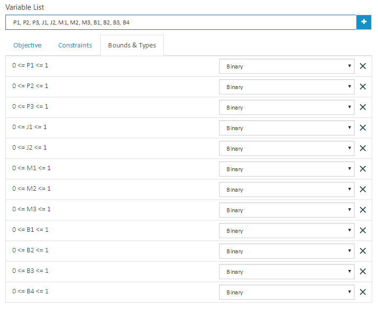
To specify that each of these options is binary (it can either be selected or not selected), you would specify this information in the Bounds & Types tab of the configuration window.
An important thing to note is that the solver in R requires that all variables be on the left-hand side of anyequality/inequality signs. This is to say, although P1 + P2 + P3 == 1 is equivalent to P1 + P2 == 1 - P3, having a variable (P3) on the right side of the equality sign (==) will cause the tool to fail with the error: R.exe exit code (3221225512) indicated an error.
Specify the model from a file
If you already have a model saved in a file, you can load it into the Optimization Tool to be solved with the Specify the model from a file mode. The model file must be one of the three formats: CLPEX_LP, MathProg, or MPS_Free.
If you choose this input mode, you do not need to connect any data to the input anchors or the problem type, but you will still need to select which solver you would like to use.
Fun Fact:If you would like to see any examples of inputs in Alteryx, there is a Sample Workflow built into Designer that includes examples of each type of input underHelp > Sample Workflows > Predictive tool samples > Prescriptive Analytics > 1 Optimization Model Input Modes
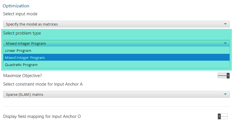
Select problem type
Once your inputs are all configured, you can specify your problem type. As mentioned in the introduction, the Alteryx Optimization Tool allows you to pick from Linear Programming, Mixed Integer Programming, and Quadratic Programming.
Which option will be best suited for your use case should have been determined in the problem set-up stage of the process.
Select Solver
After you have specified your problem type, you may have the option to select between solvers. If you are working with a Linear or Mixed Integer Program, you can choose between Glpk and Symphony.If you are working with a Quadratic Program, you will be using the Quadprog solver.
Maximize Objective?
The last thing we need to talk about in the configuration is the maximize objective option. This is simply a toggle that lets you choose between minimizing or maximizing your target objective. In a case where you are dealing with cost per unit, you will probably want to leave this toggle to the default, so that the Optimization Tool will find you a solution where the objective (cost) is minimized. However, if you are dealing with profit per unit, you will likely want to switch this toggle to maximize your potential total profit.
Outputs
The Optimization Tool will return three outputs when given a problem it is able to solve.
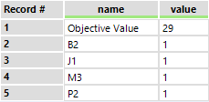
The (S) output will contain the solution:
For this problem, we see that the Optimization Tool selected P2, J1, M3, and B2 to maximize the objective (profit) to 29.
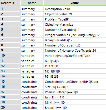
The (D) output contains three pip-separated tables of data. these tables are the Summary, Variables, and Constraints:
This data can be easily parsed out with a Filter Tool (to separate the rows for each table, based on the name column), and then a Text to Columns Toolusing apipe (|) as the delimiter. This data can be handy for developing your own reports and dashboards for the Optimization problem and returned solution.
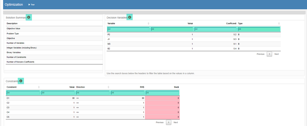
The final anchor, (I) returns an interactive dashboard of the solution:
For help navigating this dashboard, try clicking on the information icons, and filtering with the search boxes at the top of each table.
With this guide, I hope you feel more comfortable configuring the Alteryx Optimization Tool. If you would like to see a video demonstrating this process, please see this recorded Live Training. For additional help with your specific optimization task, please don't hesitate to post to the Designer Discussion forum with your problem, theoretical setup (how you are thinking about approaching the problem), and what you have developed so far in Alteryx. Never fear, the Community is here to help you!
By now, you should have expert-level proficiency with the Optimization Tool! If you can think of a use case we left out, feel free to use the comments section below! Consider yourself a Tool Master already? Let us know atcommunity@alteryx.comif you’d like your creative tool uses to be featured in the Tool Mastery Series.
Stay tuned with our latest posts everyTool Tuesdayby followingAlteryxon Twitter! If you want to master all the Designer tools, considersubscribingfor email notifications.
- Mark as Read
- Mark as New
- Bookmark
- Permalink
- Notify Moderator
I have version 2018.3 and I am having trouble locating this macro. Any advice?
- Mark as Read
- Mark as New
- Bookmark
- Permalink
- Notify Moderator
Hi @npeereboom,
The Optimization tool can be found in the Prescriptive tool category. If you are not seeing this category in Designer, please check that you have installed the Alteryx Predictive tools, which are a separate download and installation from Alteryx Designer. The Optimization tool is R-based and included in the Predictive Tools installation.
Thanks!
Sydney
- Mark as Read
- Mark as New
- Bookmark
- Permalink
- Notify Moderator
Hi Sydney, thank you very much for this article! It has given me a good starting point to leverage this tool.
- Mark as Read
- Mark as New
- Bookmark
- Permalink
- Notify Moderator
SydneyF It's a great post, thank you! I also have seen in the documentation that there is option for sensititvity analysis in linear proggramming. How can I set and see it?
- Mark as Read
- Mark as New
- Bookmark
- Permalink
- Notify Moderator
Hi @Konstantina_Gk,
Thank you for your question. Currently, sensitivity analysis is not available in the Optimization tool. If this is something you would like to see added in a future release, please consider posting to our Designer Ideas Forum. Our product managers are active here, and always looking for great new features to add to the products.
Thanks,
Sydney
- Mark as Read
- Mark as New
- Bookmark
- Permalink
- Notify Moderator
Per Designer Discussion, depending on the way you define your constraints, it's sometimes important that the rows in the O input be in the same order as the rows in the A input and that the columns in the A input be in the same order as the rows in the B input. The names are for human readability.
- Mark as Read
- Mark as New
- Bookmark
- Permalink
- Notify Moderator
Great article! I read this after watching the recorded video (hosted by Joe Miller) which covered the Linear Program option and this article answered the questions on the Mixed Integer Prg and the Sparse (SLAM) Matrix perfect.
Thank you!
- Mark as Read
- Mark as New
- Bookmark
- Permalink
- Notify Moderator
Great explanation. Thanks. When I tried running the sample workflow, I got an R.exe error. I am using 2021.2.3 version, and my R version is 4.0.4. Does it need any configuration update to make the workflow run?
Thanks.
RudolphC
- Mark as Read
- Mark as New
- Bookmark
- Permalink
- Notify Moderator
Nice read here! It will take time to get the configurations down, but articles like this one are immensely helpful.
-
2018.3
1 -
2023.1
1 -
API
2 -
Apps
7 -
AWS
1 -
Configuration
4 -
Connector
4 -
Container
1 -
Data Investigation
11 -
Database Connection
2 -
Date Time
4 -
Designer
2 -
Desktop Automation
1 -
Developer
8 -
Documentation
3 -
Dynamic Processing
10 -
Error
4 -
Expression
6 -
FTP
1 -
Fuzzy Match
1 -
In-DB
1 -
Input
6 -
Interface
7 -
Join
7 -
Licensing
2 -
Macros
7 -
Output
2 -
Parse
3 -
Predictive
16 -
Preparation
16 -
Prescriptive
1 -
Python
1 -
R
2 -
Regex
1 -
Reporting
12 -
Run Command
1 -
Spatial
6 -
Tips + Tricks
1 -
Tool Mastery
99 -
Transformation
6 -
Visualytics
1
- « Previous
- Next »
