What is R?
In addition to being a letter of the alphabet, R is also a powerful statistical programming language. People around the world from students to experienced data scientists and cutting edge researchers in many fields use it. It’s not too difficult to do many basic tasks in R, but those tasks won’t be the focus of this post. The tools/macros we’ll discuss in this series of posts all use the Alteryx R tool in some capacity. The Alteryx R tool allows you to use the R language within an Alteryx workflow, app, or macro. We won’t be learning about the direct use of the R tool today, but if you want to learn more about using it, please comment on this post and ask me to write another post about it! This is my first EngineWorks post, so I’m still figuring out what topics Alteryx users want to hear more about.
How do I access these tools?
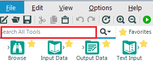
First, you’ll need to make sure that R and these tools are installed. To do so, open up Alteryx Designer, click “Options” on the toolbar and then choose “Download Predictive Tools.” These tools may not show up on your tool palette, but recall that you can find any tools using the “Search All Tools” option in the upper left corner next to the “Favorites” tab.
How do I know which tool(s) to use for my prediction problem?
Step one: What’s the Problem?
First, you need to decide whether you have a classification or a regression problem. You can count the number of potential outcomes in a classification problem. For example, trying to predict whether a customer will buy a certain item is a classification problem because it only involves two outcomes (either the customer buys the item or not). Predicting whether a person will drive, bike, walk, or take public transit to work is also a classification problem, because it involves four possible outcomes (the four different potential modes of transportation). The set of possible outcomes of a regression problem, on the other hand are continuous. Intuitively, a continuous variable can take any value within a certain range. For example, predicting people’s heights is a regression problem, because adult heights could range anywhere from 21.5 inches to 107.1 inches. For the rest of this post, we’ll assume you’re solving a classification problem, but a future post about regression tools may be forthcoming!
Step two: What’s in the data?
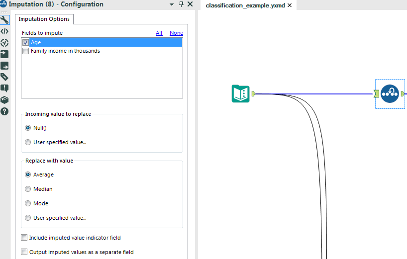
Next, you need to consider your data. For example, if you have missing values in your data, you need to take extra care in selecting your predictive tool(s). Some of the tools, such as the Forest Model, Neural Network, Support Vector Machines (SVM), and Logistic Regression, do not allow you to use data with missing values. If you have data with missing values and wish to use one of these tools, you have two options. The first option is to use an Imputation tool to impute your missing values before using one of these tools. In this example, an entry is missing from the Age field. So we impute it before using the aforementioned tools on our data. If you’ve never used the Imputation Tool before, you might want to play around with it for a bit. (Note: It’s in the Preparation category if you’re having trouble finding it.) But the basic idea behind this tool is pretty simple. If you have data with null records (or another type of record you don’t want), the Imputation Tool allows you to replace these records with the field average, median, mode, or another value you can choose to specify. In this example, we impute with the average.
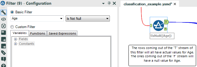
The second option for dealing with missing data is to use a Filter tool to remove the missing values.
Now, the bad news at this point is that both of these approaches for dealing with missing data have their flaws. The main limitation of imputing null values is that it can cause our model to be based on incorrect information. In the example above, the missing age value was imputed as 45. But what if this person was actually 18? Then we could have gotten a very different model from the “true” model resulting from the complete data set. The primary flaw of filtering out null data points, on the other hand, is that it can bias our data. Suppose in our example that we had a few more missing age values. Let’s say that all of these values were missing because older respondents did not feel comfortable disclosing their ages in this survey. Then basing our model only on complete records (which is what happens when we filter out nulls) will bias it towards younger respondents.
Luckily, we don’t always have to choose one of these imperfect options if we have missing data. There are other classification tools that handle missing data all on their own. The two included in the Predictive toolset are the Decision Tree and the Naïve Bayes Classifier. However, you need to include at least two predictor fields in order to use the Naïve Bayes Classifier.
In addition to missing data, you should consider the presence of outliers in your data. Some models, such as Support Vector Machines, Decision Trees, and the Forest Model aren’t affected very strongly by outliers and are thus a good choice to use in data sets with them.
Finally you should consider the number of features in your data. As mentioned above, the Naïve Bayes Classifier requires that you include at least two predictor fields. However, other methods are better suited to data sets with a smaller number of predictors. For example, Support Vector Machines, Logistic Regression, and Neural Networks can overfit your data if you have too many features. (There are ways to choose the parameters for these models so that overfitting is less likely, but those methods are outside the scope of this post.) Overfitting occurs when your model conforms too well to the data you used to train it and doesn’t generalize well to new data. It is especially likely to happen with models that use a large number of features. A test frequently used to detect overfitting is called cross-validation. Unfortunately, Alteryx Designer does not have a built-in cross-validation tool at the time of this writing (Version 10.1). However, one is currently in the pipeline, so stay tuned for an announcement about its release!
If you have a data set with many features, you should consider using a tree-based tool such as the Decision Tree or a Forest Model. With the Decision Tree, you can limit the number of features used by changing any of the following settings under the Model Customization tab as directed:
- Increasing the minimum number of records needed to allow for a split
- Increasing the allowed minimum number of records in a terminal node
- Decreasing the maximum allowed depth of any node in the final tree
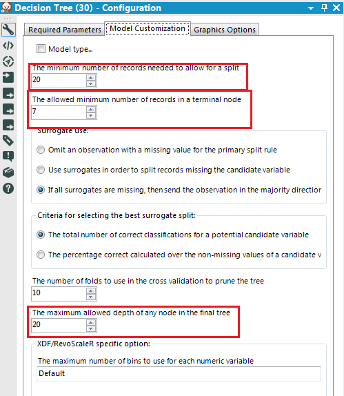
Try playing around with various combinations of these three options and seeing what kind of model you obtain!
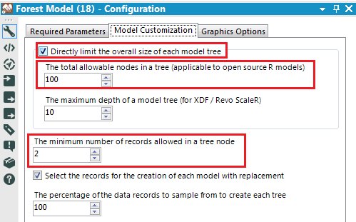
Forest Models are even better for limiting overfitting, because their design is customized for this very purpose. (A mathematical explanation of their design is beyond the scope of this post, but I’d be happy to provide one in the comments section for any interested readers.) The default settings for the Forest Model will likely result in a model that is not overfitted. However, if you’re still concerned about overfitting, you can also customize the model parameters in the following ways under the Model Customization tab. These steps will likely limit the number of features used by your model:
- Check the box for “Directly limit the overall size of each node tree.” Then decrease the total allowable nodes in a tree.
- Increase the minimum number of records allowed in a tree node.
How do I understand the output of the tool(s) I chose?
All of the classification tools have at least two outputs: an O output for the model object, and an R object for a report about the model. If this is your first time using the Predictive tools, you can probably ignore the O output for now. However, you should attach a Browse tool to the R output so you can actually see the report about your model. Here’s a partial screenshot from the R output on the Support Vector Machines tool:
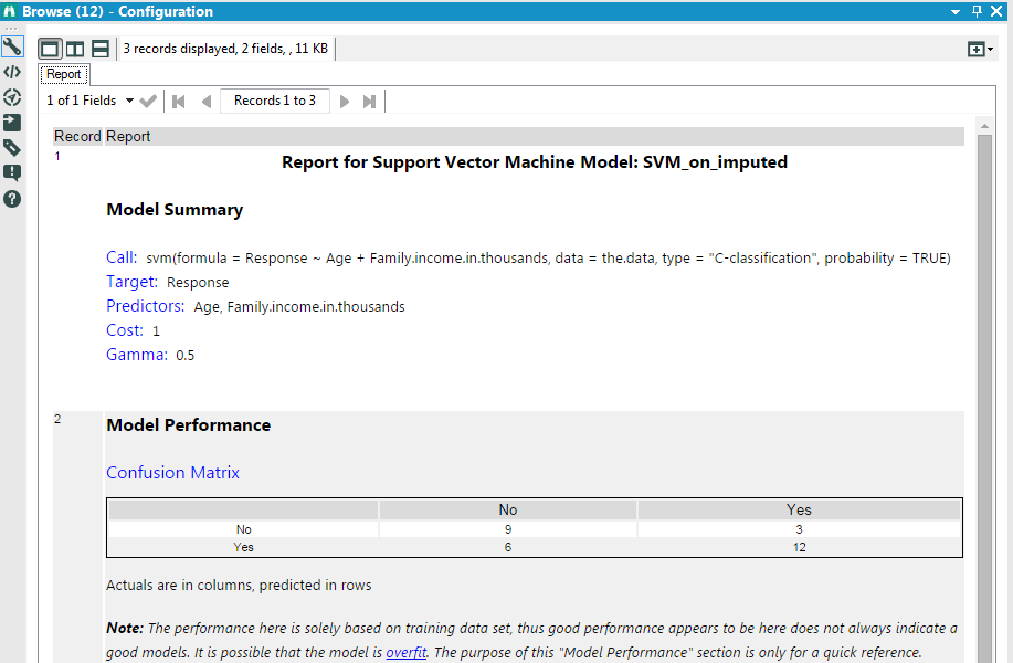
Under Model Summary, the call is a copy of the R code used within the Support Vector Machines tool in order to generate the model. The target is the variable being predicted, and the predictors are the variables used to predict the target. The values for cost and gamma are parameters for the model. They can be user-specified, but I’d suggest letting the tool select them for you if this is your first time using the Predictive tools. (If you want a more detailed explanation of these parameters, please ask for one in the comments!) The confusion matrix displays how many members of each class the model assigned to the various possible classes. In this example, the model assigned 9 members of the “No” class correctly (the top left column) and 6 incorrectly (the bottom left column). It also classified 3 members of the “Yes” class incorrectly (the top right column) and 12 correctly (the bottom right column).
Additionally, the report for Support Vector Machines contains an SVM classification plot. This plot is colored based on the region associated with each class to which the Support Vector Machines model would assign data.
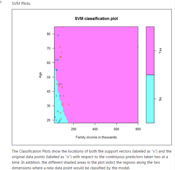
In this example, the pink/purple region corresponds to “Yes” responses, and the teal region corresponds to “No” response. So for example, a 30-year-old whose family made $200,000 would be predicted as a “Yes” response because such a person would fall into the pink/purple region.
The other classification models all generally have similar “Model Summary” sections as well as a Confusion Matrix, in addition to output that is unique to the model type. If you have questions about the output from other models, feel free to ask them in the comments section!
Well, that’s finally the end of what I have to say (for now, at least). Feel free to take a look at the attached workflow if you want a more hands-on example of using these tools. Try changing some of the input data and even model parameters if you’re feeling adventurous! Thanks for reading, and please leave your feedback in the comments section! My next post will likely be about evaluating your model’s accuracy, but I’m open to other suggestions if you’d like to learn about something else. Finally, don’t forget to visit the new Predictive District on the Gallery if you want to check out even more predictive tools!