Alteryx Designer Desktop Discussions
Find answers, ask questions, and share expertise about Alteryx Designer Desktop and Intelligence Suite.- Community
- :
- Community
- :
- Participate
- :
- Discussions
- :
- Designer Desktop
- :
- Re: FIFO Calculation with multiple products
FIFO Calculation with multiple products
- Subscribe to RSS Feed
- Mark Topic as New
- Mark Topic as Read
- Float this Topic for Current User
- Bookmark
- Subscribe
- Mute
- Printer Friendly Page
- Mark as New
- Bookmark
- Subscribe
- Mute
- Subscribe to RSS Feed
- Permalink
- Notify Moderator
I am trying to calculate the cost of sales under First-in-first-out method. The cost could be calculated by excel, which is in column N in the "Results" file. However, I am not sure how I could use Alteryx to do the same thing.
Any help is much appreciated. Thanks in advance.
Cheers,
Austin
Solved! Go to Solution.
- Labels:
-
Transformation
- Mark as New
- Bookmark
- Subscribe
- Mute
- Subscribe to RSS Feed
- Permalink
- Notify Moderator
Hi @grossal,
Sorry that I miss the negative sign in my last reply.
The formula in the excel is =SUMPRODUCT(--(-SUM($L$3:L4)>I$3:I4),-SUM($L$3:L4)-$I$3:I4,K$3:K4)-SUM($M$3:M3)
So the first part should be as below.
-SUM($L$3:L4) > I3 -> 100 > 0 -> True -> 1
-SUM($L$3:L4) > I4 -> 100 > 100 -> False -> 0
Apologies for the confusion
- Mark as New
- Bookmark
- Subscribe
- Mute
- Subscribe to RSS Feed
- Permalink
- Notify Moderator
The logic of the last formula may not seem intuitive. I would definitely love to see other approach that would be more straightforward to get the results.
I try to divide the formula into different parts below. You may also use "Evaluate formula" function in excel to simplify the formula as well.
Let's take the formula in cell M4 as an example:
=SUMPRODUCT(--(-SUM($L$3:L4)>$I$3:I4),-SUM($L$3:L4)-$I$3:I4,$K$3:K4)-SUM($M$3:M3)
1st part: --(-SUM($L$3:L4)>$I$3:I4)
= {IF -SUM($L$3:L4) > I3, THEN = 1, ELSE 0; IF -SUM($L$3:L4) > I4, THEN = 1, ELSE 0}
= {1;0}
2nd part: -SUM($L$3:L4)-$I$3:I4,$K$3:K4
= {-SUM($L$3:L4) - I3 ; -SUM($L$3:L4) - I4} , {$K$3 ; K4}
= {100-0 ; 100-100}, {8 ; 0}
= {100 ; 0} , {8 ; 0}
3rd part: -SUM($M$3:M3)
= 0
So, adding all parts will equal to SUMPRODUCT( {1;0} , {100;0} , {8;0} ) - 0
= (1*100*8 + 0*0*0) - 0
= 800
Using the same logic, the formula in cell M9 =SUMPRODUCT(--(-SUM($L$6:L9)>$I$6:I9),-SUM($L$6:L9)-$I$6:I9,$K$6:K9)-SUM($M$6:M8)
=SUMPRODUCT ( {1;1;1;0} , {150;50;50;0} , {150;0;10;0} ) - SUM(M6:M8)
= ( 1*150*150 + 1*50*0 + 1*50*10 + 0*0*0 ) - 15000
= 8000
The logic is to calculate the cumulative total cost of sales starting from the beginning by SUMPRODUCT(--(-SUM($L$6:L9)>$I$6:I9),-SUM($L$6:L9)-$I$6:I9,$K$6:K9) and subtract the previous cost of sales up to the last transaction with -SUM($M$6:M8). So, the remaining balance would be the non-cumulative cost of sales for that particular transaction. Hope this is clearer.
- Mark as New
- Bookmark
- Subscribe
- Mute
- Subscribe to RSS Feed
- Permalink
- Notify Moderator
The logic of the last formula may not seem intuitive. I would definitely love to see other approach that would be more straightforward to get the results.
I try to divide the formula into different parts below. You may also use "Evaluate formula" function in excel to simplify the formula as well.
Let's take the formula in cell M4 as an example:
=SUMPRODUCT(--(-SUM($L$3:L4)>$I$3:I4),-SUM($L$3:L4)-$I$3:I4,$K$3:K4)-SUM($M$3:M3)
1st part: --(-SUM($L$3:L4)>$I$3:I4)
= {IF -SUM($L$3:L4) > I3, THEN = 1, ELSE 0; IF -SUM($L$3:L4) > I4, THEN = 1, ELSE 0}
= {1;0}
2nd part: -SUM($L$3:L4)-$I$3:I4,$K$3:K4
= {-SUM($L$3:L4) - I3 ; -SUM($L$3:L4) - I4} , {$K$3 ; K4}
= {100-0 ; 100-100}, {8 ; 0}
= {100 ; 0} , {8 ; 0}
3rd part: -SUM($M$3:M3)
= 0
So, adding all parts will equal to SUMPRODUCT( {1;0} , {100;0} , {8;0} ) - 0
= (1*100*8 + 0*0*0) - 0
= 800
Using the same logic, the formula in cell M9 =SUMPRODUCT(--(-SUM($L$6:L9)>$I$6:I9),-SUM($L$6:L9)-$I$6:I9,$K$6:K9)-SUM($M$6:M8)
= SUMPRODUCT ( {1;1;1;0} , {150;50;50;0} , {150;0;10;0} ) - SUM(M6:M8)
= ( 1*150*150 + 1*50*0 + 1*50*10 + 0*0*0 ) - 15000
= 8000
The logic is to calculate the cumulative total cost of sales starting from the beginning by SUMPRODUCT(--(-SUM($L$6:L9)>$I$6:I9),-SUM($L$6:L9)-$I$6:I9,$K$6:K9) and subtract the previous cost of sales up to the last transaction with -SUM($M$6:M8). So, the remaining balance would be the non-cumulative cost of sales for that particular transaction. Hope this is clearer.
- Mark as New
- Bookmark
- Subscribe
- Mute
- Subscribe to RSS Feed
- Permalink
- Notify Moderator
My earlier reply got deleted after editing. Trying to repost below
The logic of the last formula may not seem intuitive. I would definitely love to see other approach that would be more straightforward to get the results.
I try to divide the formula into different parts below. You may also use "Evaluate formula" function in excel to simplify the formula as well.
Let's take the formula in cell M4 as an example:
=SUMPRODUCT(--(-SUM($L$3:L4)>$I$3:I4),-SUM($L$3:L4)-$I$3:I4,$K$3:K4)-SUM($M$3:M3)
1st part: --(-SUM($L$3:L4)>$I$3:I4)
= {IF -SUM($L$3:L4) > I3, THEN = 1, ELSE 0; IF -SUM($L$3:L4) > I4, THEN = 1, ELSE 0}
= {1;0}
2nd part: -SUM($L$3:L4)-$I$3:I4,$K$3:K4
= {-SUM($L$3:L4) - I3 ; -SUM($L$3:L4) - I4} , {$K$3 ; K4}
= {100-0 ; 100-100}, {8 ; 0}
= {100 ; 0} , {8 ; 0}
3rd part: -SUM($M$3:M3)
= 0
So, adding all parts will equal to SUMPRODUCT( {1;0} , {100;0} , {8;0} ) - 0
= (1*100*8 + 0*0*0) - 0
= 800
Using the same logic, the formula in cell M9 =SUMPRODUCT(--(-SUM($L$6:L9)>$I$6:I9),-SUM($L$6:L9)-$I$6:I9,$K$6:K9)-SUM($M$6:M8)
= SUMPRODUCT ( {1;1;1;0} , {150;50;50;0} , {150;0;10;0} ) - SUM(M6:M8)
= ( 1*150*150 + 1*50*0 + 1*50*10 + 0*0*0 ) - 15000
= 8000
The logic is to calculate the cumulative total cost of sales starting from the beginning by SUMPRODUCT(--(-SUM($L$6:L9)>$I$6:I9),-SUM($L$6:L9)-$I$6:I9,$K$6:K9) and subtract the previous cost of sales up to the last transaction with -SUM($M$6:M8). So, the remaining balance would be the non-cumulative cost of sales for that particular transaction. Hope this is clearer.
- Mark as New
- Bookmark
- Subscribe
- Mute
- Subscribe to RSS Feed
- Permalink
- Notify Moderator
We are getting closer! @AustinLeung
If you sum up every cost in the excel per stock and in my version - both are equal. I am currently trying to figure out the last details to make them exactly equal.
e.g.
Apple [Excel] = 800
Apple [Me] = 800
Banana [Excel] = 15000+8000 = 23000
Banana [Me] = 22500 + 500 = 23000
...
- Mark as New
- Bookmark
- Subscribe
- Mute
- Subscribe to RSS Feed
- Permalink
- Notify Moderator
Great! So glad to hear that. Would you mind sharing the file so that I could have a look on what you are doing? Thanks a lot!
- Mark as New
- Bookmark
- Subscribe
- Mute
- Subscribe to RSS Feed
- Permalink
- Notify Moderator
@grossal, I guess we could use Run Total as the last step?
- Mark as New
- Bookmark
- Subscribe
- Mute
- Subscribe to RSS Feed
- Permalink
- Notify Moderator
Hey @AustinLeung , hey @grossal ,
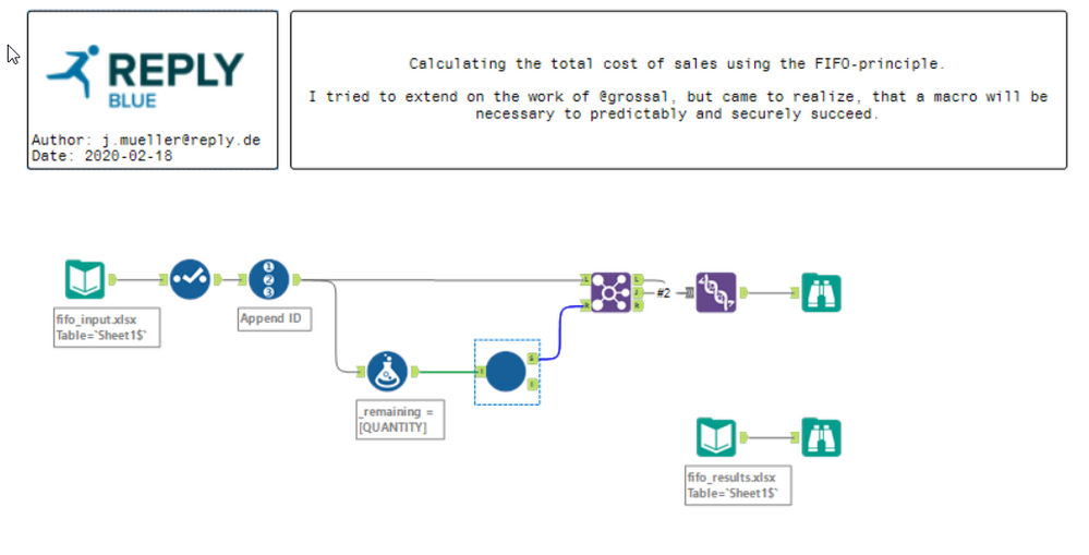
I really liked your problem, since it is quite tricky and intriguing. At a first glance, I thought I could solve this using only standard tools, like @grossal tried.
I actually succeeded in creating a solution for your example data, but shortly before posting I came to realize that this won't work for more complex scenarios.
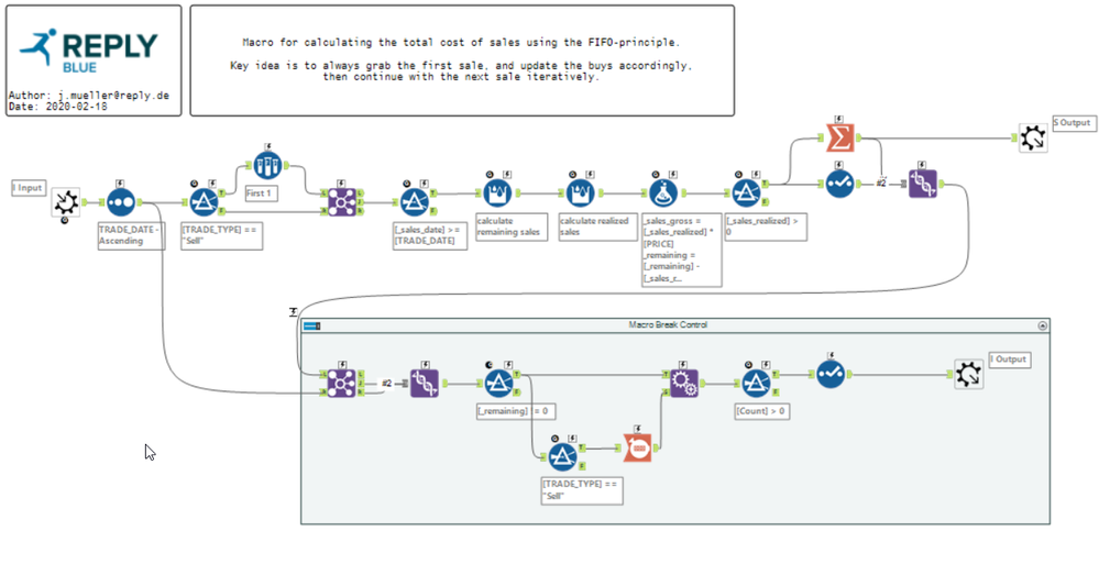
Therefore I introduced (nearly) the same code in an iterative macro which, for each iteration takes one sale and collects its respective buys.
After calculating the amount of sold units, the remaining stock of the buys is updated and the sale is removed from the list.
The tool box in the lower part of the macro serves mostly to control the macros flow.
I hope this could solve your problem.
Best,
Johannes
(Blue Reply)
- Mark as New
- Bookmark
- Subscribe
- Mute
- Subscribe to RSS Feed
- Permalink
- Notify Moderator
Hi Muller,
I have been trying to use @grossal approach but also find that the logic does not work for more complex scenarios.
I am still trying to understand your work but I have tested a few samples and that works!
I will try to apply the model to my actual data and see if all is fine. Thank you very much for your help!
- Mark as New
- Bookmark
- Subscribe
- Mute
- Subscribe to RSS Feed
- Permalink
- Notify Moderator
As @reply_mueller said, this was a really interesting problem, possibly even one for @JoeS to have a look at for a weekly challenge! Ever since you first posted it, I've been mulling it over, scribbling notes on random pieces of paper, mumbling away to myself, etc.
As Johannes also realized, I knew that an iterative macro would solve it, but I was obsessed with finding another way.
I finally settled on the following idea. Convert all the buy events and sell event to rows with a quantity of 1. Then the FIFO principle becomes easier to implement.
My solution attached below
-
Academy
6 -
ADAPT
2 -
Adobe
204 -
Advent of Code
3 -
Alias Manager
78 -
Alteryx Copilot
25 -
Alteryx Designer
7 -
Alteryx Editions
94 -
Alteryx Practice
20 -
Amazon S3
149 -
AMP Engine
252 -
Announcement
1 -
API
1,208 -
App Builder
116 -
Apps
1,360 -
Assets | Wealth Management
1 -
Basic Creator
15 -
Batch Macro
1,558 -
Behavior Analysis
246 -
Best Practices
2,693 -
Bug
719 -
Bugs & Issues
1 -
Calgary
67 -
CASS
53 -
Chained App
268 -
Common Use Cases
3,823 -
Community
26 -
Computer Vision
85 -
Connectors
1,426 -
Conversation Starter
3 -
COVID-19
1 -
Custom Formula Function
1 -
Custom Tools
1,936 -
Data
1 -
Data Challenge
10 -
Data Investigation
3,486 -
Data Science
3 -
Database Connection
2,220 -
Datasets
5,221 -
Date Time
3,227 -
Demographic Analysis
186 -
Designer Cloud
740 -
Developer
4,369 -
Developer Tools
3,528 -
Documentation
526 -
Download
1,037 -
Dynamic Processing
2,937 -
Email
927 -
Engine
145 -
Enterprise (Edition)
1 -
Error Message
2,256 -
Events
198 -
Expression
1,868 -
Financial Services
1 -
Full Creator
2 -
Fun
2 -
Fuzzy Match
711 -
Gallery
666 -
GenAI Tools
3 -
General
2 -
Google Analytics
155 -
Help
4,706 -
In Database
966 -
Input
4,291 -
Installation
360 -
Interface Tools
1,900 -
Iterative Macro
1,094 -
Join
1,957 -
Licensing
252 -
Location Optimizer
60 -
Machine Learning
259 -
Macros
2,862 -
Marketo
12 -
Marketplace
23 -
MongoDB
82 -
Off-Topic
5 -
Optimization
750 -
Output
5,252 -
Parse
2,327 -
Power BI
228 -
Predictive Analysis
936 -
Preparation
5,167 -
Prescriptive Analytics
205 -
Professional (Edition)
4 -
Publish
257 -
Python
855 -
Qlik
39 -
Question
1 -
Questions
2 -
R Tool
476 -
Regex
2,339 -
Reporting
2,431 -
Resource
1 -
Run Command
575 -
Salesforce
277 -
Scheduler
411 -
Search Feedback
3 -
Server
629 -
Settings
933 -
Setup & Configuration
3 -
Sharepoint
626 -
Spatial Analysis
599 -
Starter (Edition)
1 -
Tableau
512 -
Tax & Audit
1 -
Text Mining
468 -
Thursday Thought
4 -
Time Series
431 -
Tips and Tricks
4,187 -
Topic of Interest
1,126 -
Transformation
3,726 -
Twitter
23 -
Udacity
84 -
Updates
1 -
Viewer
3 -
Workflow
9,976
- « Previous
- Next »


