Background information & the standard Output Data approach
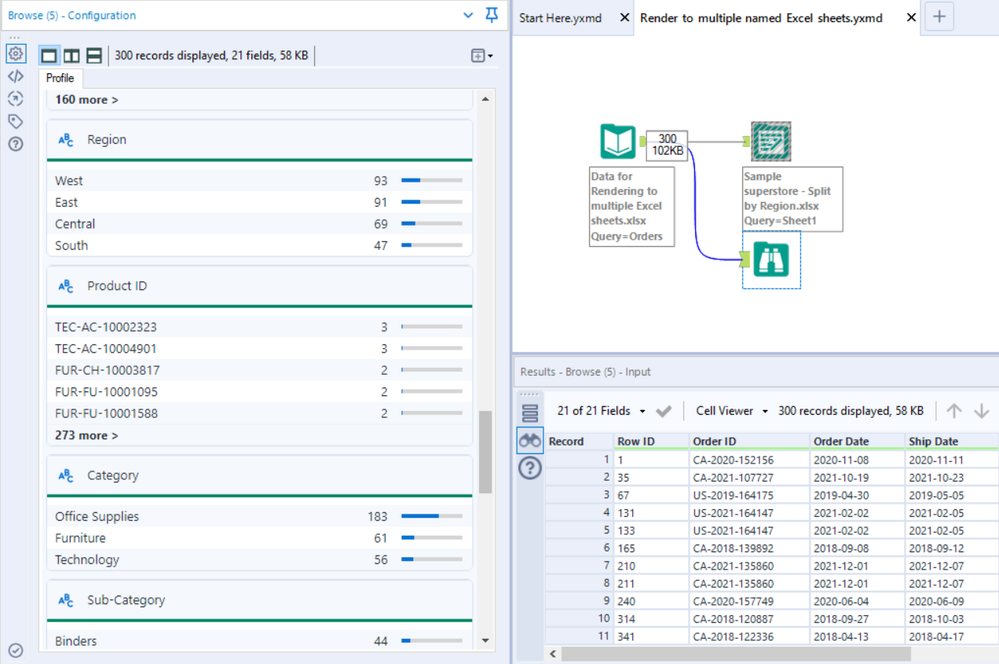
Whilst outputting the results of a workflow, we often find ourselves publishing to an Excel spreadsheet. At times, this also involves splitting our data into separate sheets within the Excel file. When dealing with regular, unformatted results, the standard Output Data tool does a great job of allowing us to handle this. For example, if we want to split out the following dataset (Tableau users will be more than familiar with good ol’ Sample Superstore!) into Regions, we can see from a quick Browse that the resulting worksheet should include 4 separate tabs - West, East, Central and South.
Now, as mentioned above, all we have to do to achieve this result is configure our Output Data tool in the following way:
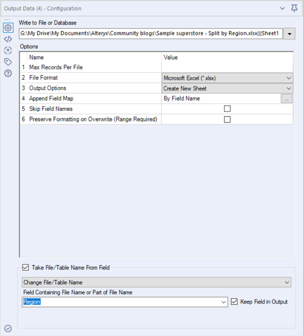
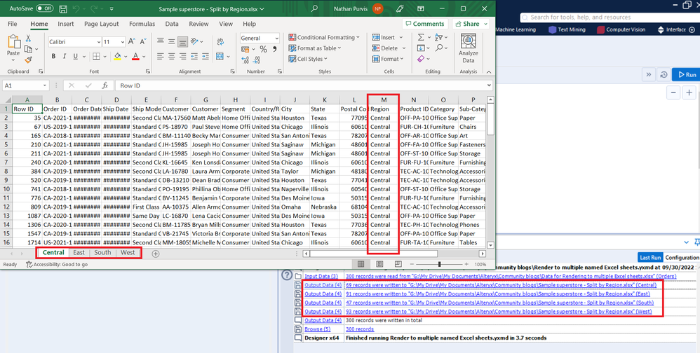
Once you’ve chosen your desired output location and a name for the file, you can put whatever you want in the sheet name as this essentially becomes a placeholder, and the emphasis shifts to the bottom section where we tick Take File/Table Name From Field and then select Change File/Table Name. Here we then just need to select the field which will split our data, which in this case is [Region]. The remaining option to ‘Keep Field in Output’ will do exactly what it says - I often split on custom fields I have created just to generate sheet names, and so I regularly untick this. However, if you’re using a field that forms part of the actual data - like this example - I’d keep this selected; otherwise Alteryx will remove the column from the output. When we run the workflow, we now get an Excel spreadsheet that is nicely split up into our 4 regions as expected:
Why do we need the Render method?
So, what’s the point of this blog? Well, as pointed out previously, this only works for unformatted data, i.e. things that haven’t gone through the reporting palette and been converted into reporting snippets. From here on out, we’ll look at how to achieve the same outcome as above, using a Render tool instead to push out our results, as the process is a little more nuanced and requires a few extra steps and configurations. For this example, we’ll be placing our data into tables before outputting to a tab for each region.
Setting up the Table tool
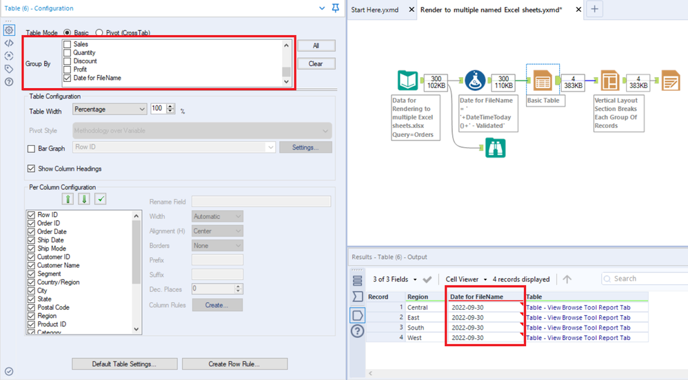
The first step is to bring our Table tool onto the canvas, and this is where we begin telling Alteryx how to group our data. As mentioned, we’re again going to have a tab for each [Region] in the dataset, and so that is our field to Group By:
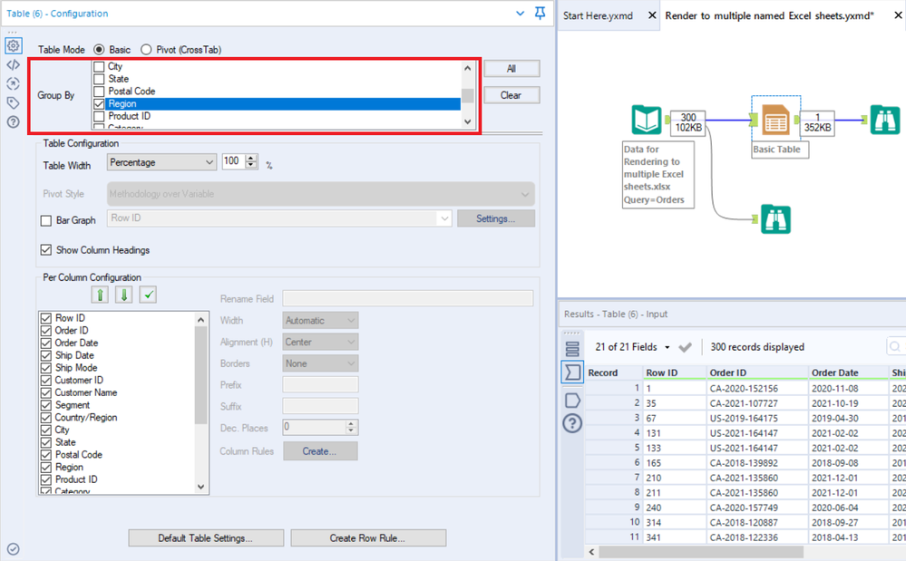
A quick run shows us that the table has been split, as expected, into 4 records, i.e. a single reporting snippet (Table) for each Region:
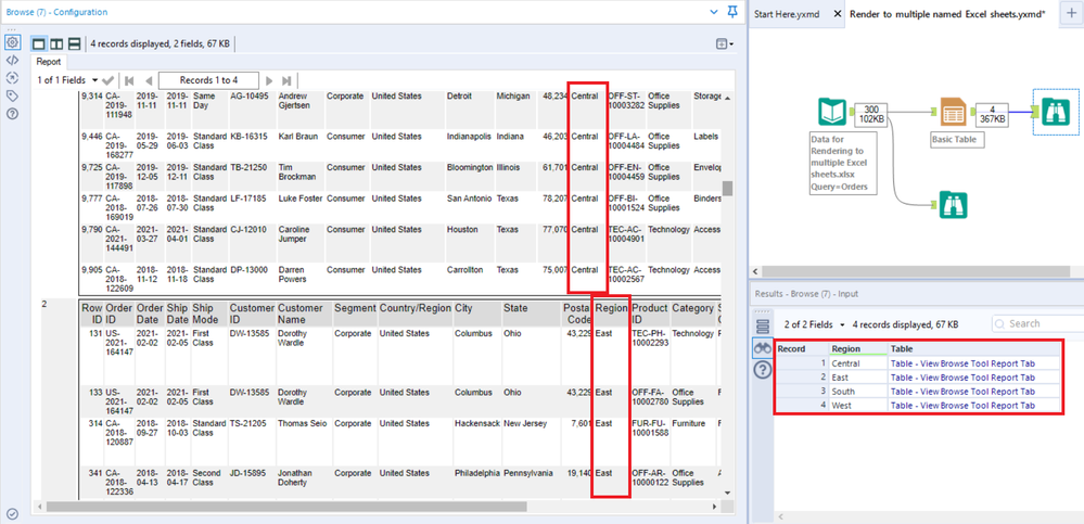
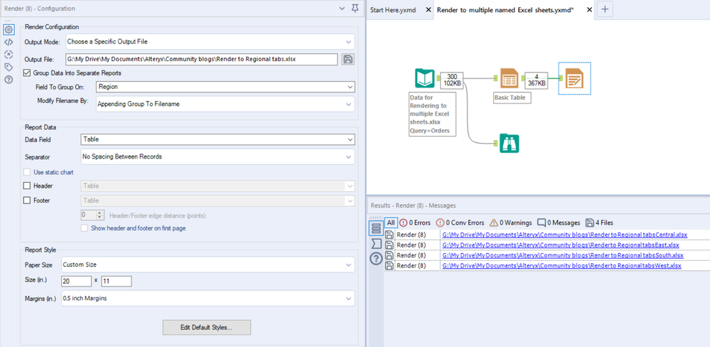
Great, so we can just Render now, referencing the [Region] field… right? Well, unfortunately, the tool doesn’t allow us to do that as Output Data does - the only options when using grouped outputs here all involve changes to the filename. Therefore if we try going down this route, we end up with 4 different files altogether rather than just 4 different tabs:
Setting up the Layout tool
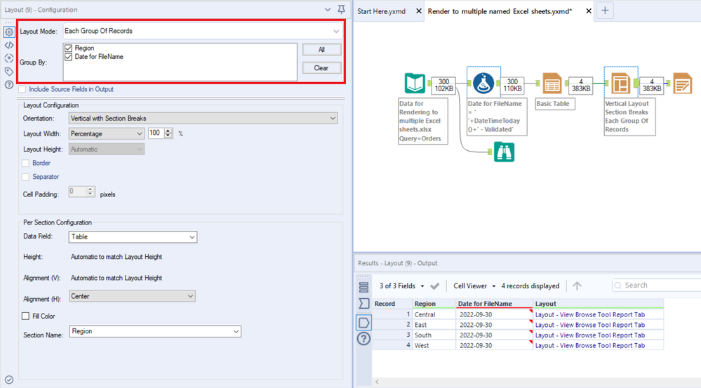
To get around this, we need to involve a Layout tool before we move to Render. When it comes to the configuration, we need to select Each Group Of Records as the Layout type and select our Group By field, which happens to be [Region] in this case. After that, be sure to use Vertical with Section Breaks as the Orientation and select the grouping field for the Section Name:
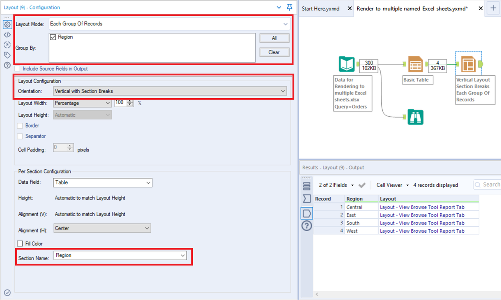
The way we set up the section break and name here is essential for what we’re trying to achieve; for reports like PDFs and word documents, a section break represents a new page. However, when outputting to an Excel file, a section break marks the start of a new tab. The fact that we can name these sections then gives us our Regional tab names as opposed to them just coming out as ‘Sheet1’, ‘Sheet2’ etc.
Setting up the Render tool
Following the Layout tool, we can now finally move to outputting our Excel file via the Render tool! The setup here is actually very simple due to the fact that everything has been prepared in the previous tools. First of all, unless you just want the output to be a temporary file that you can look over, you’ll need to change the Output Mode to Choose a Specific Output File. After that, click on the little save icon and navigate to your target directory before setting a file name and type as usual (in this case, obviously, .xlsx). The Layout should automatically be populated as the Data Field. However, if for some reason it isn’t, be sure to set that. The final thing to check is that, especially if you have large tables, the Paper Size is large enough to handle your output - starting off this rendering process by outputting to a temporary Excel file is the best way to test this. In this instance, my table was too large for the ‘Letter’ size that is selected by default, and I have therefore set custom dimensions:
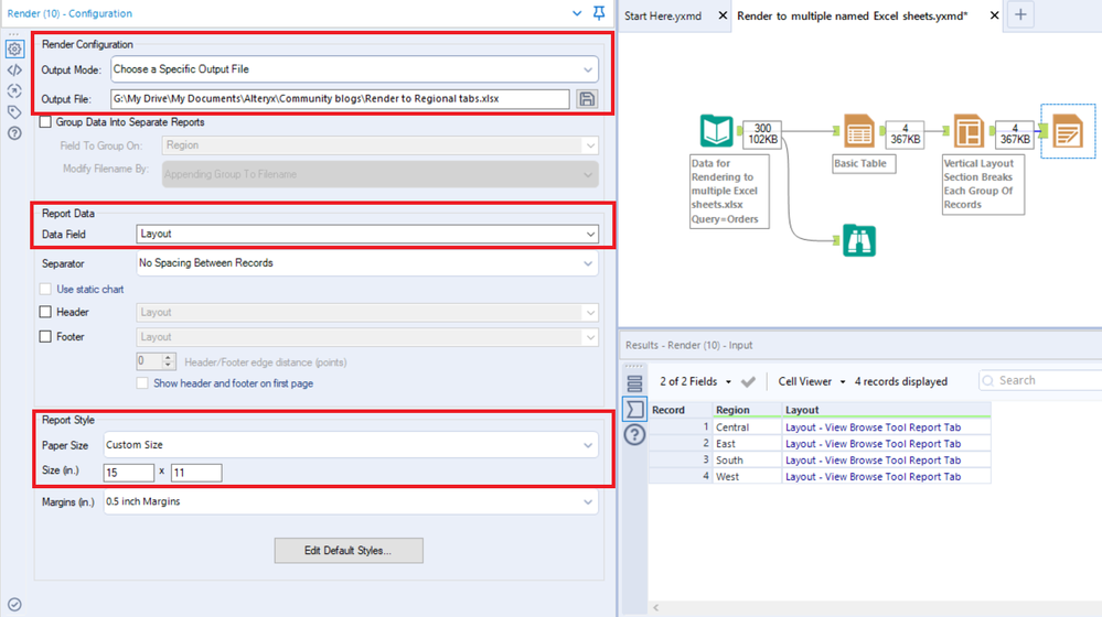
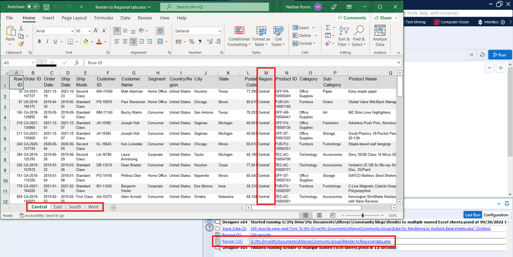
Running this workflow will now output to a single Excel workbook. Unlike Output Data where each of the tabs are shown in the results pane, this time the section break is happening behind the scenes and we’ll just get a single Render message. However, when we open up the file we can see that the data has been split and tabs named exactly as we wish:
Additional information & tips
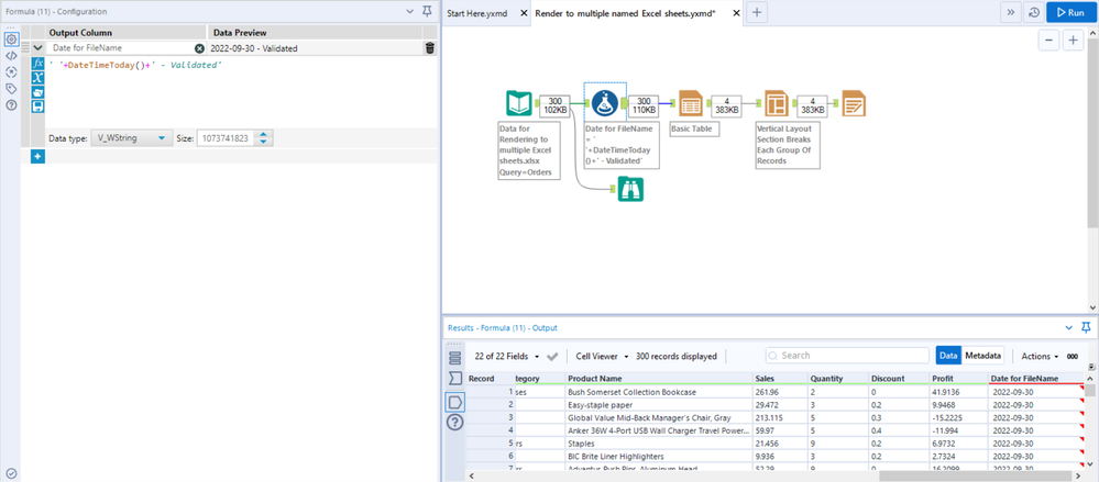
As an extra to this blog, one thing I often see requests for is the use of dynamic parts of a file name, i.e., today’s date. Here I’ll show how you can maintain this render but add additional parts to the workbook’s name. You may remember earlier that the options available to us in the Group Data Into Separate Reports dropdown all involved changes to the filename. Well, guess what? We’re going to leverage that. The steps to this are incredibly simple and just involve us creating a custom string that we can then add to the start/end of the filename or replace it entirely. For the sake of a quick example, I’m just going to add today’s date and the word ‘Validated’ to the output file. The first stage is just using a Formula tool to build this addition:
Much like we did with [Region] before, we need to ensure that this newly-created field is ticked in the Group By options of our Table & Render tools so that it remains as a field alongside the reporting snippets throughout:
Because of the way we have set up this custom string (with a space followed by the date/word ‘Validated’), this is designed to go at the end of the filename. Obviously, if you wanted to prepend this, then you’d re-order this to fit. The final process here is to tick the Group Data Into Separate Reports option that we left untouched before. We then select the field we built within the Formula tool and, at least for my example, choose Appending Group To Filename:
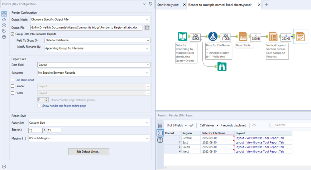
This time when we run our workflow, we get the same as above, but with today’s date reflected in the filename:
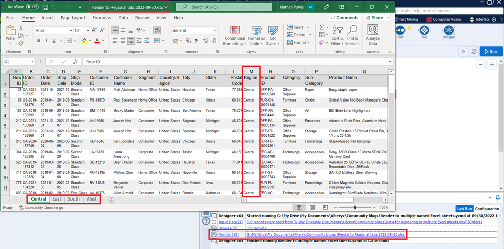
This was set up as a quick example, but you can add many dynamic parts to the filename, including values from fields that will split your data into multiple workbooks if that’s also what you want.
In terms of Tab names, you can also customise these more and add dynamic parts; you just need to bring them through in the Group By of the reporting tools and remember to set that field as the Section Name in the Layout tool.
Hopefully, this blog has helped to explain the process of being able to split your table renders into separate Excel files without having to make any sacrifices on sheet or file names! If you need any further explanation or support, then please feel free to get in touch.
Additional Resources:
Alteryx & Excel Guide
Output to multiple sheets within an Excel file
How to output multiple tabs within a single Excel file based on a field name