Data Science
Machine learning & data science for beginners and experts alike.- Community
- :
- Community
- :
- Learn
- :
- Blogs
- :
- Data Science
- :
- Using Alteryx Tools for the Occupancy Detection Pr...
- Subscribe to RSS Feed
- Mark as New
- Mark as Read
- Bookmark
- Subscribe
- Printer Friendly Page
- Notify Moderator
In 2017 the US’s primary energy consumption was equal to about 97.7 quadrillion British Thermal Units (BTU). That's 97,728,000,000,000,000!
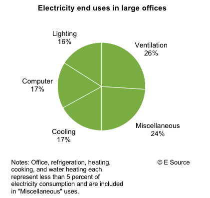
The occupancy detection problem is a well-known problem in the sensor industry that can be applied to help reduce major energy consumption in buildings. The chart below shows that about 60% – 70% of energy used in office buildings can be attributed to HVAC (Heating, Ventilation, and Air Conditioning).
Average energy use data – OUC (Business Energy Advisor)
If you are hoping to reduce HVAC costs in your office, having a reliable model that can turn off/on these HVAC systems can help reduce the usage of electricity.
In this blog, I am going to tackle the Occupancy Detection Problem by using Alteryx to create a logistic regression model. First, I am going to create a model generated with the R-Based Logistic Regression Tool (included in the Predictive Tools Installation) and then compare it with the model created in the Python Tool (introduced in version 2018.3).
Since this binary classification problem is used to predict whether a room is occupied based on environmental factors such as temperature, humidity, CO2 and related measures, I found a perfect dataset from the UCI Machine Learning repository. This dataset includes variables such as date-time, temperature, humidity, humidity ratio, light, CO2, and occupancy. The main objective of this project is to estimate the probability of whether or not a room is occupied based on the sensor data.
Variable information
- Date Time: Year-Month-Day hh:mm:ss
- Temperature in Celsius.
- Relative Humidity as a percentage.
- Light measured in Lux.
- CO2 measured in parts per million (ppm).
- Humidity Ratio which was a derived quantity from temperature and relative humidity in
.
7. Occupancy as either 0 for not occupied or 1 for occupied.
The dataset is available in a .txt format, but we can bring it in Alteryx as a .csv with a comma as a delimiter.
The three files are as follows:
- txt (test): From 2015-02-02 14:19:00 to 2015-02-04 10:43:00
- txt (train): From 2015-02-04 17:51:00 to 2015-02-10 09:33:00
- txt (val): From 2015-02-11 14:48:00 to 2015-02-18 09:19:00
As you can see, these datasets are not continuous in time, and do have a couple of gaps. Because of these missing periods, a time series model may not be suitable for this dataset.
Creating the model with the Logistic Regression predictive tool
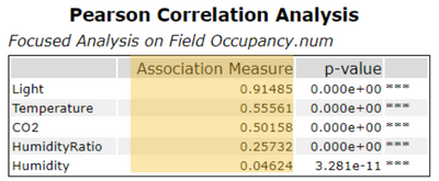
Before I start my analysis, I want to use the Association Analysis tool to learn if any of the variables are correlated with one another. Knowing how the predictor variables relate to the target variable (Occupancy) will help me with variable selection.
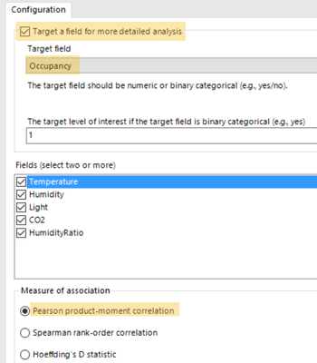
This chart tells me that Light and Occupancy variables are closely correlated and suggest they have a fairly strong relationship. Because of this relationship, I know now that light is an important variable to include to create a more accurate model. This also suggests that the room in which the environmental variables were recorded may have had a light sensor that turned the internal lights on when the room was occupied. It could also mean that light is recorded during the daylight hours (e.g., as sunshine through windows) and the rooms are occupied during each day.
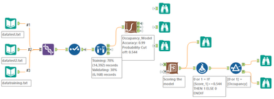
Below is how I have decided to set up my workflow.
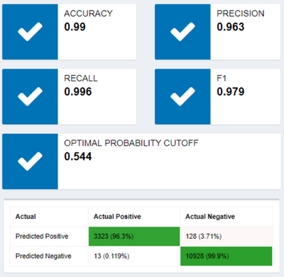
I am using the create samples tool to create a 70/30 split of the records. 70% of the records will be used to train the model, while the other 30% will be used to validate the model. After selecting the target variable (Occupancy) and the predictor variables (Temperature, Humidity, Light, CO2, and Humidity Ratio), the model has an Accuracy score of 0.99 with an optimal probability cutoff of 0.544 (this is the suggested threshold at which to divide predicted 0’s and 1’s). Looking at the model summary below (included in the I anchor of the Logistic Regression Tool), the predicted positive vs actual positive was 96.3% (3323 records) while only 3.71% (128) of the records weren’t predicted correctly. On the other side, the predicted negative vs actual negative was 99.9% while only 0.119% (13) of the records weren’t predicted correctly. In laymen’s terms, this model is better at predicting 0’s (not occupied) than 1’s (occupied). Regardless, these are very good results for an initial model.
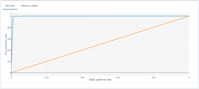
My ROC (Receiver Operating Characteristic) curve also indicates a strong model. The ROC chart, included in the Interactive (I) Output is a plot of the true positive rate against the false positive rate for the different possible cut points of the diagnostic test.
What that basically means is that the closer the curve flows to the left-hand border and the top border of the ROC space, the more accurate the test it. The closer the curve comes to the 45 degree diagonal of the ROC space, the less accurate the test. In laymen’s terms, you can consider the area under the curve as a measure of accuracy.
A closer look at the predictor variables in R
We can take a further look at each variable, and see what impact it has on the occupancy in isolation. The idea here is that we might not need all the variables to predict occupancy, and only one or two variable(s) might be sufficient. This may help simplify the sensor requirements in the HVAC systems as well. I went ahead and isolated each variable.
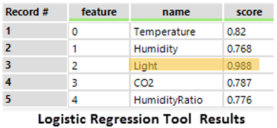
We can see that the Light variable has a score of 0.988 and is required to attain 99% accuracy on this dataset.
Creating the model in Python
Let’s now compare the Logistic Regression Tool to the Python model.
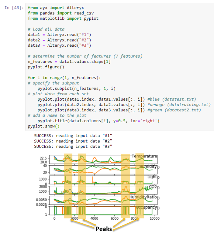
First, as I did when preparing the data for the Logistic Regression Tool, I am going to combine the datasets into one single stream using the union tool and then connect it to the Python Tool. I am also going to bring in the 3 different datasets separately because I want to plot the datasets independently to see if there are trends with the variables.
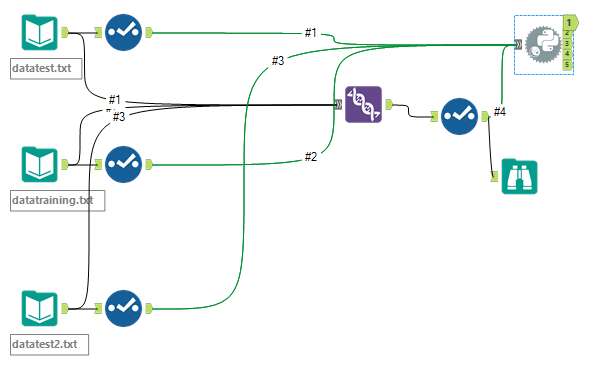
Using the pyplot functions in the tool’s interface to generate and display a plot, we get the graph below.
This plot depicts that when a person is in the room, some of the variables rise and create a peak.
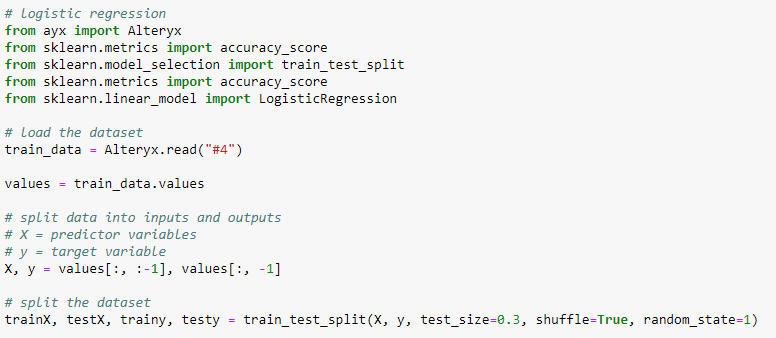
Now we will use the combined dataset (#4) to create a logistic regression model. We are again going to do a 70/30 split. We are going to use the 70% (14,392) of the dataset to train the model and 30% (6,168) of the dataset to validate the model. Although the percentage of the records used to train versus test the model is the same as what we did for the Logistic Regression Tool, because the sampling is randomized, the actual data used to train the Python-based model is likely slightly different from the data that was used to train the R-based model.
Our training dataset (14,392 records) is:
- trainX: predictor variable
- trainy: target variable
Our validating dataset (6,168 records) is:
- testX: predictor variable
- testy: target variable
Scikit-learn is a set of Python modules for machine learning and data mining. This library is your go-to for statistical and predictive modeling and evaluation. Here is a summary of the sklearn.linear_model.LogisticRegression (for reference):
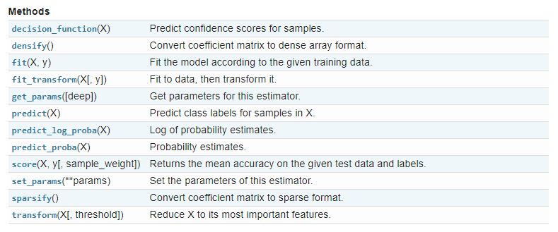
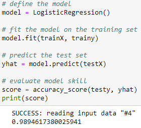
After we split the dataset, we want to create our model. In Python, the first step is to define the model (model = LogisticRegression()). Next, we want to fit the model on the training dataset (trainX, trainy) using model.fit(trainX, trainy). The next step is to use the model.predict on the testX variable to create the results (yhat). Finally, we want to evaluate the model using the accuracy_score, comparing the actual results (testy) versus the predicted result (yhat).
As you can see, our score was 0.9894 (0.99 approx.), which is a pretty good score and an impressive result.
A closer look at the predictor variables in Python
Looking at the graph from earlier, we can see a clear relationship between the times the room was occupied and relative peaks in the environmental variables. This makes sense - the problem is straightforward and we saw pretty good results from the model (score = 0.9894).
Similar to the Logistic Regression tool, we can take a further look at each variable and see what impact it has on the occupancy in isolation.

Writing out the score for each variable using Alteryx.write(df,1) gives us the results below:
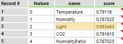
We can see that the Light variable has a score of 0.9834 and is required to attain 99% accuracy on this dataset. Comparing the results from both models in isolation:
Here we see that both results are very similar. The variable we want to focus on is the light variable, both having an accuracy score of 0.98. This means that if we decide to just pick Light as the predictor variable, our model will receive an accuracy score of 0.98. The minor difference between both scores could be because of the packages (Python: Scikit Learn vs R; glm) that are being used for calculations, or the differences in training data (as the 70% sample was random between the two methods).
Conclusion
There are several things we can conclude from the data set.
- The model created in Python versus the model created in the Logistic Regression tool have very similar results (Score of 0.9894 vs 0.99, respectively). The difference could be caused because of the different packages used to creating both models, or the training data. The Python tool is from the Python package Sci-kit learn, (sklearn.linear_model) while the Logistic Regression tool is coded in R (with the glm package). Nevertheless, both models gave us impressive results.
- Perhaps adding additional variables to the dataset such as acoustic, ultrasonic sensors that measure sound and motion detection could help us create a more accurate model. Perhaps some of those variables are better correlated than light?
- We can try different algorithms, perhaps a random forest model? I encourage you guys to try it out and post your results in the comments!
Hopefully, this blog was beneficial and I was able to show you how one can leverage advanced data analytics and predictive modeling in real-world scenarios.
An important side note that most people forget
The Logistic Regression tool was able to give me more out of the box insights regarding the model than what I coded in the Python Tool. Within the Python code, I would have to create all the graphs, charts, analysis (ROC curve, performance, density plots etc.) myself from scratch. If I did not know how to create these in Python, I would have to look up and research the extra functions and plotting packages. With the premade tool in Alteryx, I do not have to do any of that. I simply selected my target and predictor variables and voila, my results from the model are beautifully graphed and I can share them with other data scientists for further evaluation.
In Python, on the other hand, I can write custom code from scratch allowing for better model customization per use case. I was able to model and score in one tool (Python tool) rather than using 2 different tools in Alteryx (Logistic Regression and Score tool).
Now if I want to deploy this model in a production instance, I can deploy it within Alteryx Promote. Alteryx Promote provides a solution for deploying and managing predictive models and scoring data with real-time decision APIs. It allows data scientists and analytics teams to deploy predictive models to production faster — and more reliably — without writing any custom deployment code. I will touch upon Promote in a different blog!
You must be a registered user to add a comment. If you've already registered, sign in. Otherwise, register and sign in.
