Data Science
Machine learning & data science for beginners and experts alike.- Community
- :
- Community
- :
- Learn
- :
- Blogs
- :
- Data Science
- :
- Tidying up with PCA: An Introduction to Principal ...
- Subscribe to RSS Feed
- Mark as New
- Mark as Read
- Bookmark
- Subscribe
- Printer Friendly Page
- Notify Moderator
Principal component analysis (PCA) is a technique for dimensionality reduction, which is the process of reducing the number of predictor variables in a dataset.
More specifically, PCA is an unsupervised type of feature extraction, where original variables are combined and reduced to their most important and descriptive components.
The goal of PCA is to identify patterns in a data set, and then distill the variables down to their most important features so that the data is simplified without losing important traits. PCA asks if all the dimensions of a data set spark joy, then gives the user the option to eliminate ones that do not.
PCA is a very popular technique, but it is often not well understood by the people implementing it. My goal with this blog post is to provide a high-level overview of why to use PCA, as well as how it works.
The Curse of Dimensionality (Or, Why Bother with Dimensionality Reduction?)
The curse of dimensionality is a collection of phenomena that generally describes that, as dimensionality increases, the manageability and effectiveness of the data tend to decrease. On a high level, the curse of dimensionality is related to the fact that as dimensions (variables/features) are added to a data set, the average and minimum distance between points (records/observations) increase.

Creating good predictions becomes more difficult as the distance between the known points and the unknown points increases. Additionally, features in your data set may not add much value or predictive power in the context of the target (independent) variable. These features do not improve the model but increase noise in the dataset, as well as the overall computational load of the model.
Because of the curse of dimensionality, dimensionality reduction is often a critical component of analytic processes. Particularly in applications where the data has high-dimensionality, like computer vision or signal processing.
When collecting data or applying a data set, it is not always apparent or easy to know which variables are important. There is not even a guarantee that the variables you picked or were provided are the right variables. Furthermore, in the era of big data, the sheer number of variables in a data set can get out of hand and even become confusing and deceptive. This can make it difficult (or impossible) to select meaningful variables by hand.
Have no fear, PCA looks at the overall structure of the continuous variables in a data set to extract meaningful signals from the noise in the data set. It aims to eliminate redundancy in variables while preserving important information.

How PCA Works
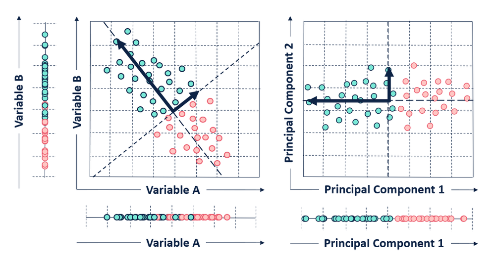
PCA originally hails from the field of linear algebra. It is a transformation method that creates (weighted linear) combinations of the original variables in a data set, with the intent that the new combinations will capture as much variance (i.e., the separation between points) in the dataset as possible while eliminating correlations (i.e., redundancy).
PCA creates the new variables by transforming the original (mean-centered) observations (records) in a dataset to a new set of variables (dimensions) using the eigenvectors and eigenvalues calculated from a covariance matrix of your original variables.
That is a mouthful. Let’s break it down, starting with mean-centering the original variables.
The first step of PCA is centering the values of all of the input variables (e.g., subtracting the mean of each variable from the values), making the mean of each variable equal to zero. Centering is an important pre-processing step because it ensures that the resulting components are only looking at the variance within the dataset, and not capturing the overall mean of the dataset as an important variable (dimension). Without mean-centering, the first principal component found by PCA might correspond with the mean of the data instead of the direction of maximum variance.
Once the data has been centered (and possibly scaled, depending on the units of the variables) the covariance matrix of the data needs to be calculated.
Covariance is measured between two variables (dimensions) at a time and describes how related the values of the variables are to one another: e.g., as the observed values of variable x increase is the same true for variable y? A large covariance value (positive or negative) indicates that the variables have a strong linear relationship with one another. Covariance values close to 0 indicate a weak or non-existent linear relationship.

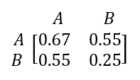
Covariance is always measured in two dimensions. If you are dealing with more than two variables, the most efficient way to make sure you get all possible covariance values is to put them into a matrix (hence, covariance matrix). In a covariance matrix, the diagonal is the variance for each variable, and the values across the diagonal are a mirror for one another because each combination of variables is included in the matrix twice. This is a square, symmetric matrix.
In this example, the variance of variable A is 0.67, and the variance of the second variable is 0.25. The covariance between the two variables is 0.55, which is mirrored across the main diagonal of the matrix.
Because they are square and symmetrical, covariance matrixes are diagonalizable, which means an eigendecomposition can be calculated on the matrix. This is where PCA finds the eigenvectors and eigenvalues for the data set.
An eigenvector of a linear transformation is a (non-zero) vector that changes by a scalar multiple of itself when the related linear transformation is applied to it. The eigenvalue is the scalar associated with the eigenvector. The most helpful thing I’ve found to understanding eigenvectors and values is seeing an example (if this isn't making sense, try watching this matrix multiplication lesson from Khan Acadamy).

In this example, 
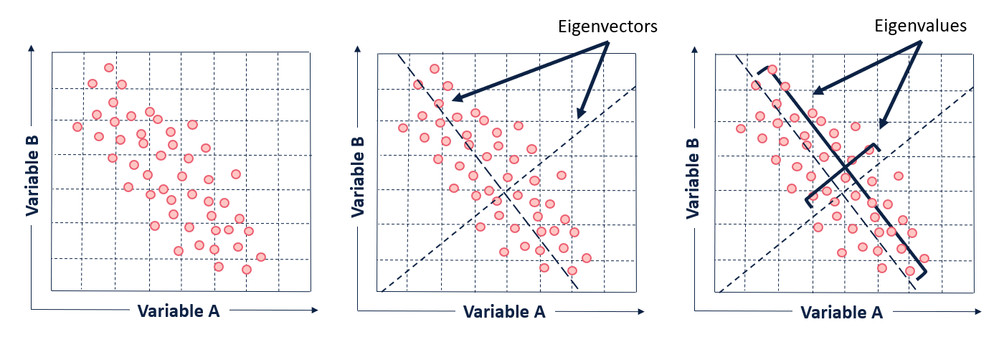
In the context of understanding PCA at a high level, all you really need to know about eigenvectors and eigenvalues is that the eigenvectors of the covariance matrix are the axes of the principal components in a dataset. The eigenvectors define the directions of the principal components calculated by PCA. The eigenvalues associated with the eigenvectors describe the magnitude of the eigenvector, or how far spread apart the observations (points) are along the new axis.
The first eigenvector will span the greatest variance (separation between points) found in the dataset, and all subsequent eigenvectors will be perpendicular (or in math-speak, orthogonal) to the one calculated before it. This is how we can know that each of the principal components will be uncorrelated with one another.
If you’d like to learn more about eigenvectors and eigenvalues, there are multiple resources scattered across the internet with exactly that purpose. For the sake of brevity, I am going to avoid attempting to teach linear algebra (poorly) in a blog post.
Each eigenvector found by PCA will pick up a combination of variance from the original variables in the data set.

The eigenvalues are important because they provide a ranking criterion for the newly derived variables (axes). The principal components (eigenvectors) are sorted by descending eigenvalue. The principal components with the highest eigenvalues are “picked first” as principal components because they account for the most variance in the data.
You can specify returning almost as many principal components as there are variables in your original data set (typically up to n-1, where n is the number of original input variables), but most of the variance will be accounted for in the top principal components. For guidance on how many principal components to select, check out this stack overflow discussion. Or you can always just ask yourself, "Self, how many dimensions will spark joy?" (That was a joke, you should probably just use a scree plot.)

After identifying the principal components of a data set, the observations of the original data set need to be converted to the selected principal components.
To convert our original points, we create a projection matrix. This projection matrix is just the selected eigenvectors concatenated to a matrix. We can then multiply the matrix of our original observations and variables by our projection matrix. The output of this process is a transformed data set, projected into our new data space - made up of our principal components!
That's it! We have accomplished PCA.
PCA in Alteryx Designer
In Alteryx Designer, there is a Principal Components tool that performs this process, found under the Predictive Grouping tool category.
The Principal Components tool uses the R function prcomp() from the R stats package. Fun fact, the Principal Components tool in Designer calculates its components with a slightly different (less intuitive to explain) method called singular value decomposition (SVD). SVD is preferred because it tends to have slightly better numerical accuracy than the method described in this post, but conceptually the outcome is the same. If you’d like to learn more about SVD specifically, check out the Stack Exchange discussions: What is the intuitive relationship between SVD and PCA and Relationship between SVD and PCA and How to use SVD to perform PCA?
Assumptions and Limitations
There are a few things to consider before applying PCA.
Normalizing the data prior to performing PCA can be important, particularly when the variables have different units or scales. You can do this in the Designer tool by selecting the option Scale each field to have unit variance.
PCA assumes that the data can be approximated by a linear structure and that the data can be described with fewer features. It assumes that a linear transformation can and will capture the most important aspects of the data. It also assumes that high variance in the data means that there is a high signal-to-noise ratio.
Dimensionality reduction does result in a loss of some information. By not keeping all the eigenvectors, there is some information that is lost. However, if the eigenvalues of the eigenvectors that are not included are small, you are not losing too much information.
Another consideration to make with PCA is that the variables become less interpretable after being transformed. An input variable might mean something specific like “UV light exposure,” but the variables created by PCA are a mishmash of the original data and can’t be interpreted in a clear way like “an increase in UV exposure is correlated with an increase in skin cancer presence.” Less interpretable also means less explainable, when you're pitching your models to others.
Strengths
PCA is popular because it can effectively find an optimal representation of a data set with fewer dimensions. It is effective at filtering noise and decreasing redundancy. If you have a data set with many continuous variables, and you aren’t sure how to go about selecting important features for your target variable, PCA might be perfect for your application. In a similar vein, PCA is also popular for visualizing data sets with high-dimensionality (because it's hard for us meager humans to think in more than three dimensions).
Additional Resources
My favorite tutorial (which includes an overview of the underlying math) is from Lindsay I. Smith at the University of Otago A tutorial on Principal Components Analysis.
Here is another great Tutorial on Principal Component Analysis from Jon Shlens at UCSD
Everything you did and didn’t know about PCA, from the blog Its Neuronal focuses on math and computation in neuroscience.
Principal Component Analysis in 3 Simple Steps has some nice illustrations and is broken down into discrete steps.
Principal Component Analysis from Jeremy Kun’s blog is a nice, succinct write up that includes a reference to eigenfaces.
A One-Stop Shop for Principal Component Analysis from Matt Brems.

A geographer by training and a data geek at heart, Sydney joined the Alteryx team as a Customer Support Engineer in 2017. She strongly believes that data and knowledge are most valuable when they can be clearly communicated and understood. She currently manages a team of data scientists that bring new innovations to the Alteryx Platform.
A geographer by training and a data geek at heart, Sydney joined the Alteryx team as a Customer Support Engineer in 2017. She strongly believes that data and knowledge are most valuable when they can be clearly communicated and understood. She currently manages a team of data scientists that bring new innovations to the Alteryx Platform.
You must be a registered user to add a comment. If you've already registered, sign in. Otherwise, register and sign in.


