Sometimes, you need to synthesize fake data.
You may not have the time or resources to acquire the data right away but need something to ask as a placeholder, you may not be able to use data for testing or demos due to privacy concerns, or you may want data that looks a specific way to prove a point.
I’m not encouraging using synthetic data for creating models to put into production or pitching something to your boss with fake data, because that is pointless and generally a bad idea. What I am saying is that sometimes when you need to run a demo, test functionality of a tool or script, or run a training session, you might need too-good-to-be-true-fakey-fake data.
And that’s where this blog post comes in. This post is 50% instructional, 50% confessional. Hopefully, I can start sleeping well again once I get this out in the open (kidding).
Recently, I was working on developing training content for an Inspire course. The course was Pre-Predictive: Fundamentals of Data Investigation, something close to my heart, and a class where the training data matters.
I wanted to use a cool animal shelter data set published by the Austin Animal Shelter, everything was going pretty well…
 http://www.austintexas.gov/department/aac
… except there aren’t many continuous variables in this data set. This is a problem when you want to teach people how to use tools like Association Analysis or Scatter Plot.
Here is the real-life story on how I created fake variables with an existing dataset. I hope you understand that the need justified the means and that you learn something along the way.
The (Real) Dataset
The Austin Animal Shelter data is comprised of two published datasets; intakes and outcomes. You can relate the intake and outcome datasets with the variable animal_id (in combination with some datetime logic because there are repeat offenders in the data, where the same sneaky puppy repeatedly breaks out of their yard and spends a few hours at the shelter before their human is able to find them again).
The variables of note in the intake dataset are found_location, intake_type, intake_condition, animal_ type, sex_upon_intake, breed, and color. The variables of note in the outcome dataset are outcome_type, outcome_subtype, sex_upon_outcome, animal_dateofbirth, and age_upon_outcome.
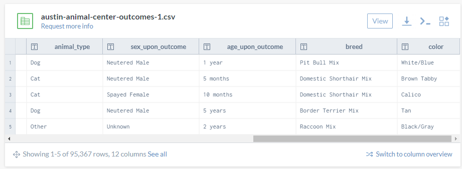
You can engineer continuous features like age upon intake and time at the shelter with the date data, but we still should have more continuous variables for data investigation purposes.
Again, this is a fabulous dataset all on its own. There are a plethora of interesting insights that can be derived from just this. But in the context of training for data investigation, where you want to get students exposed to a variety of data investigation methods, this just isn’t going to cut it. There are no continuous variables in this dataset, which is an entire category of variables that people should know how to explore and asses.
By the time I had realized that I was already in love with the data and the use case. I needed to find a way to make it work – by any means possible.
The Generated Variables
The first step in adding variables to an existing data set was to think about generated variables that might make sense in the context of the dataset. With a shelter animal dataset, logical continuous variables might include characteristics of the animal like height and weight. Because there is an intake dataset and an outcome dataset, it might even make sense to have a weight variable in each. This could allow the students in the training to visualize how height and weight relate to one another, to other variables like sex or breed, as well as how weight might change during an animal's stay at a shelter.
Sounds great! But it also sounds a little complicated to make sure that the manufactured variables line up with one another and other existing variables. Spoiler – it was – but I like to think that I made it work 🙂
How I Did It
Once I had decided to create height and weight as the continuous variables, I had to find a way to generate them that would make sense with the existing data.
With my mighty real-world knowledge, I knew that the existing data does include information related to the height and weight of an animal, such as animal type, breed, date of birth, sex, etc. I decided to start dividing out the data by variables that would cause the largest differences in height and weight. I decided animal type was the best variable to start with because cats and dogs are two different species of animals, and can be easily grouped this way.
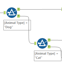
Fun fact, the Austin Animal Shelter actually takes in animals that are not cats or dogs – about 5% of the records in the dataset fall under “Bird,” “Livestock,” or “Other”: raccoons, rabbits, bats, skunks, etc.
 I wonder what a "Bat Mix" is. What does a bat mix with?
Due to the effort vs. reward tradeoff, I decided to skip generating a weight and height for these animals. I figured that the nulls in the dataset would be good experience for data investigation students anyways – here, the nulls mean that the animal is not a cat or dog, and maybe the shelter doesn’t bother with recording the height and weight of these animals (clearly not that I was too lazy to generate values for this subset of animals).
For the cats, I found the average weight and height range for an average cat, which according to Wikipedia is around 9-10 lbs., and 9-10 in., respectively. Although there is variation in average weight and height between species, there wasn’t a great internet dataset that I found on cat breed sizes, and the majority of cats in the dataset are labeled as Domestic Shorthair Mix, so average domestic cat size seemed like a fair place to start.
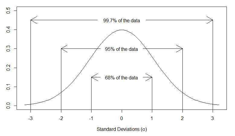
As a starting point, I decided to generate weights and heights for each cat, using a normal distribution.
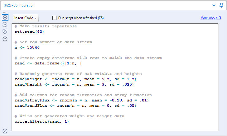
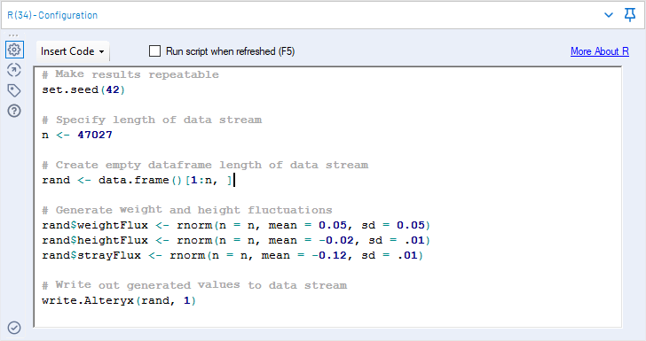
To generate the starting weights and heights, I used an R tool and a handy R function called rnorm(), which allows you to randomly generate a series of numbers with a specified population mean and standard deviation. In addition to weight and height variables, I also generated a randFlux variable and a strayFlux variable. I created the randFlux variable to simulate a difference between weight and intake and the weight at outcome. Having the exact same weight at intake and outcome would be weird, so I decided to build a random fluctuation variable to add to the generated intake weight. The strayFlux variable was generated for animals found in a sick or feral condition to reduce their weight slightly. Sad, I know, but this is a happy story where all the animals get taken care of and adopted, so we can add it back on in the weight at outcome variable.
I pushed these generated variables into my Alteryx workflow and started integrating them into the existing data set with a Join (joining on position), and then a series of if-else equations written into a Formula tool.
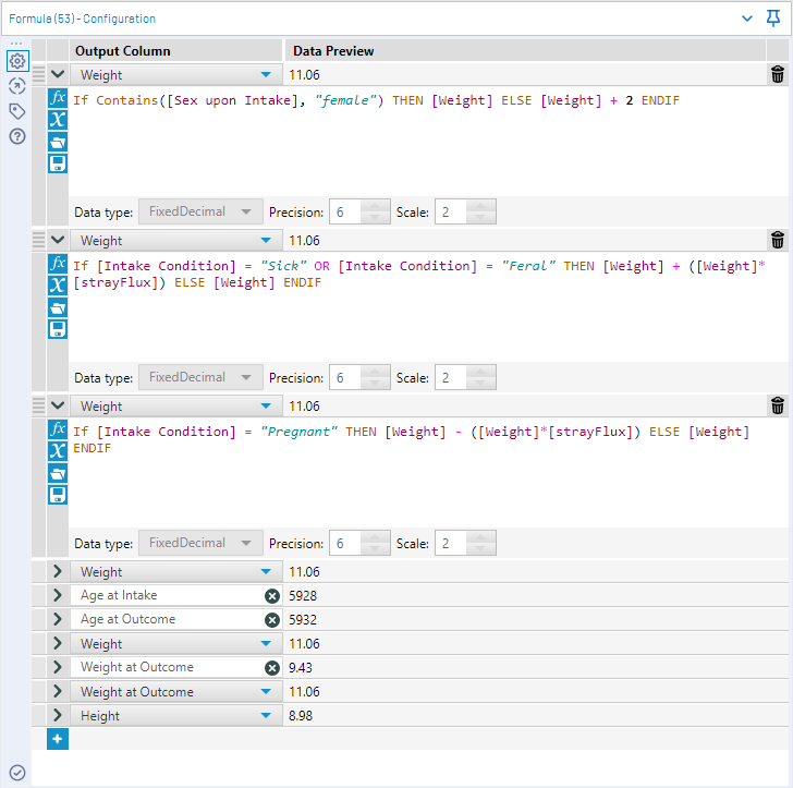
At a high level, these functions modify the randomly generated weight and height variables of the cats in the data set, depending on variables like age (kittens are smaller than cats), intake condition (pregnant cats weigh slightly more, feral cats weigh slightly less), and sex (male cats get a two pound increase). Some of these choices I tried to base on actual information (using age and an article on kitten development), others were a little more arbitrary (if a cat had "Coon" in the breed field, I added ten pounds, hooray for Maine Coons).
After all the weight and height tinkering, I used Filter tools to check for impossible values (e.g., negative or near zero values) and other data investigation tools to check that the values looked reasonable. I iterated, modifying the arguments to the R tool and Formula tool functions until what I saw made sense to me.
With the cats in a good place, I moved on to the dogs. Dogs were a little more involved than cats. As you probably know, there is a lot of variability of the height and weight of dogs depending on their breed.
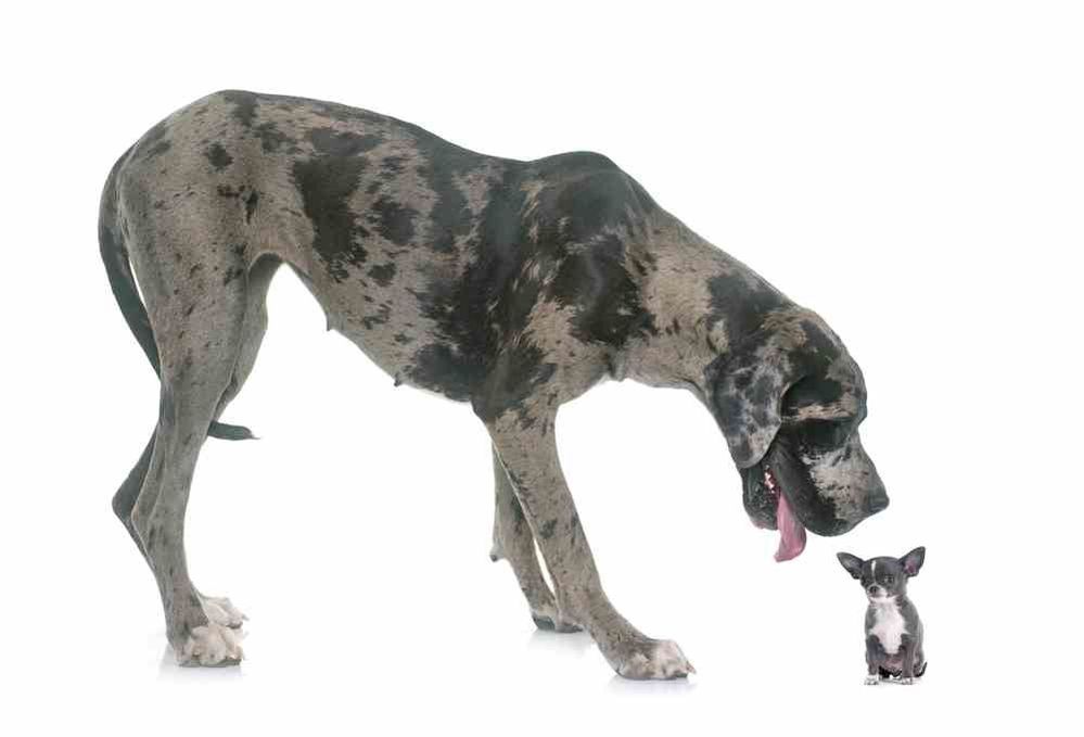
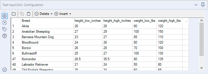
So, I brought in data from an external source.
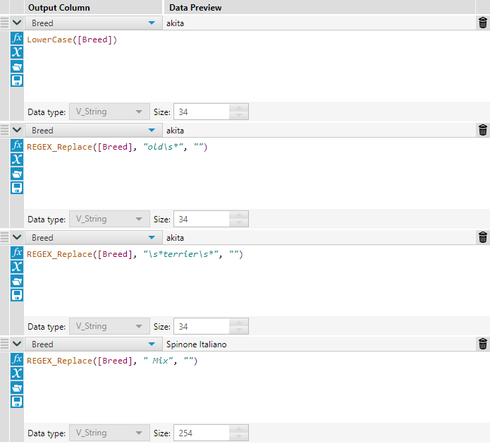
If I wanted to get really into it here, I could have gone down the rabbit hole that is Fuzzy Matching. Instead, I opted to do some light text pre-processing and then a Join.
The way the Austin Animal Shelter data is recorded, if a dog is a mixed breed they will list multiple breeds with a slash separating them. To try to track this, I did a Text to Columns parse into rows with a slash as a delimiter. Then, I joined all the shelter breed data with the weight and height ranges by breed.
I repeated this same exercise again with a space as a delimiter, trying to pick up any breeds that might have been missed due to slightly different formats (kind of like doing a waterfall with fuzzy matching). I joined all the unmatched shelter data back together and used a Summarize tool to create an average weight for each individual animal.

I then used another R tool to bring in random fluctuations in the weights and heights of the dogs.
To create a final weight and height value for each dog, I did some more Formula tool calculations, accounting for intake condition, sex, and age. For puppies, I used a slightly different growth rate calculation depending on the size of the breed they were identified as.
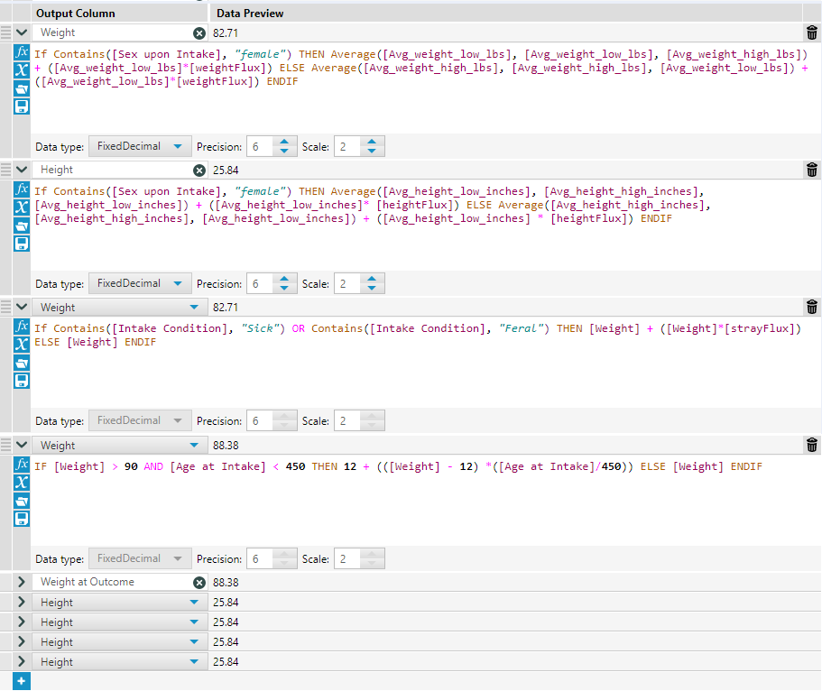
After many iterations of adjustments, I had a passable set of variables. The dataset was used in the class, and to the extent of my knowledge, none of the trainees were any the wiser, until now...
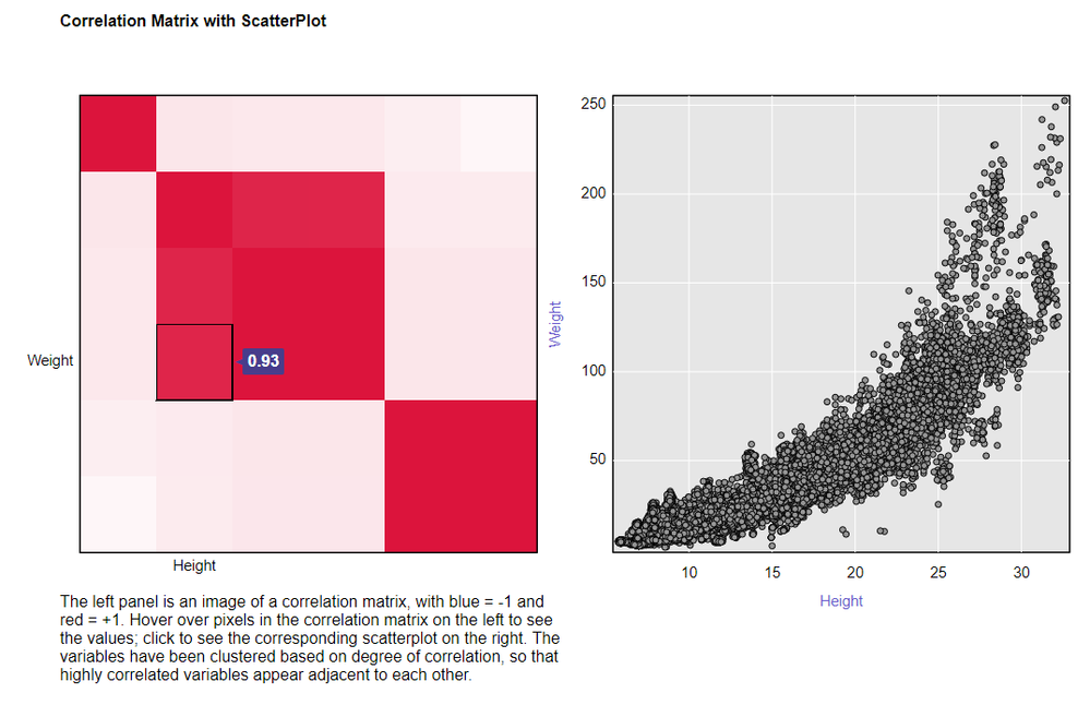
This was not a perfect attempt at generating new variables, it was effective for communicating a point and teaching. This was an involved attempt because it was important to demonstrate relationships between variables, for example, we should expect to see a strong relationship between weight and height:
A relationship between age and weight for dogs, where younger dogs weigh less and then level out:
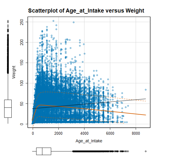
I didn't intend this, but the drop-off in the graph for big dogs as age increases makes sense to me because big dogs tend to have shorter lifespans.
There are some other relationships tucked in there, and although they are almost certainly different from what would be seen in a real data set, they are enough that a researcher could start to identify patterns and make decisions on what to keep, and what to explore - which is the whole point of data investigation.
Other Ways to Generate Data
This specific use case is pretty niche; it's not that often that you would have most of your dataset, and for some reason need to (and feel justified in) fabricating just a few new variables. There are a number of other, less hands-on ways to generate data that might better suit your use case.
There is a Python package called faker that generates fake data from scratch for you. You can read a little bit about its usage here. Another Python package for data generator is Mimesis, which was built into a Python SDK tool by the one and only @SophiaF. You can download her tool here.
The is a free tool from freeCodeCamp called DataFairy, which generates test data, that you can read about here.
For an applied approach on using Alteryx to generate Dummy data, see How to Quickly Generate Dummy Data in Alteryx from the Information Lab.
This article on Medium reviews some other Python libraries that can be used to generate dummy data for machine learning applications.
Takeaways
Fake data can be very useful, and it is an important skill in development (both software and data science) as well as for presentations.
While I was working on generating these variables, I found it was pretty easy to get caught in rabbit holes, trying to tinker the data for every special case I could think of. Although it probably (hopefully) improved the quality of the faked variables, there is a point where the effort to reward ratio was no longer viable. When generating fake data, you want the data to be representative enough of what you are simulating, but it will never be perfect because it’s not real data. Knowing what “good enough” is for your use case is critical.
Just remember, with great power comes great responsibility. Please don't use your fake data for evil.