Featured on the Data Science Portal.
Covid-19 is a black swan event.
As data analysts, what scares us most is not how convoluted the problem, but how little the data on hand. An event like this pandemic is forcing us to rebuild everything with limited data - it is for this very reason that handling missing values is more important than ever. You might ask:

Should we impute all the null rows?
Or should we just take out the variable?
Is there any imputation method other than mean?
Rather imputing once, could we impute multiple times?
How to handle missing value without bias?
This post is to answer all the questions with 2 new macros: MICE & missForest. Download the workflow & macros here, and make sure you have internet access for package installation.
No 1: Statistical Imputation with MICE

Single or Multiple Imputation (MI)
Usually, when we impute data, we think of using mean and impute once. This is called Single Imputation.
Single imputation, however, belies a severe issue: underestimation of variance (or uncertainty).
If you have one missing value out of a million rows, it makes sense to impute once. When you handle a much larger number of missing values out of a dataset, imputing a single global mean in 100 nulls across the data will heavily compromise the variance. If you are using the mean or median, it would further narrow the original potential outliers as well...
Multiple Imputation is born for this very reason, and it has become a popular topic in recent years. In a nutshell, MI creates different imputed sub-datasets (No. of Imputation), iterate the model (No. of Iteration) that converge into one complete dataset.
 https://www.researchgate.net/publication/275051563_The_rise_of_multiple_imputation_A_review_of_the_reporting_and_implementation_of_the_method_in_medical_research_Data_collection_quality_and_reporting
MICE Input
The first macro leverages MICE package. Don’t get fooled by the name, this little guy has been widely recognized in the imputation world and outperformed many mean- or regression-based algorithms. On top of the multiple imputation framework, MICE provides a variety of built-in imputation methods on a variable by variable basis.
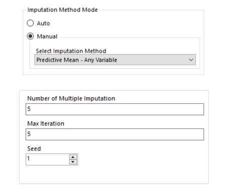
To use this macro:
1. Select columns including missing-value & non-missing for multivariate analysis.
2. Pick the Auto option under the imputation method mode. It will run by imputation method based on the data type; else, you could choose the Manual option and choose the method you prefer. Be careful that some methods require all variables to be numeric or categorical. More details can be found in the workflow.
3. Lastly, specify the number of imputations and iterations. Depends on your hardware spec, a good starting point would be 5 imputations & 5 iterations. A seed option is given for production use.
4. Run the macro and it produces 2 outputs: Completed Data (D Anchor) & Imputation Report (R Anchor)
MICE Output
The gap is filled!
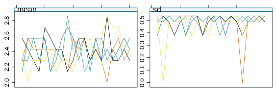
Let’s have a look at the result. One way to examine the imputation method’s effectiveness is to use the Trace Line Plot. For example, screenshots below show Contact Type in both Auto & Manual reports. Every line represents each imputed data set. We hope to see that across the iterations (X Axis), both mean & standard deviation (Y Axis) are similar but not identical since we want some variation to replicate the uncertainties.
Both means and standard deviations vary between 2.0 - 2.8 and 0 - 0.5 in these charts. However, Manual mode seems like a little bit better as the lines look less than the Auto mode, particularly we would like to see convergence in the last few rounds of iterations.
Auto:
- Method: Polytomous Regression
- No of Imputation: 5
- No of Iteration: 20
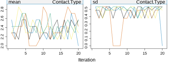
Manual:
- Method: Binary Logistic
- No of Imputation: 5
- No of Iteration: 20
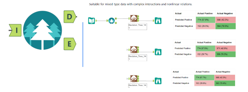
Another evaluation mechanism is to use a supervised-learning model to see which imputed dataset has higher predictive power. In this example, subscription status is our target variable, which makes it as a classification problem. Simply drag & drop a Decision Tree tool, and use Contact Type as the predictor. Below are the confusion matrices:

Based on the higher TP & TN rate, we could conclude the Manual Mode with Binary Logistic method is a better option.
That’s it for MICE. Nevertheless, this package has so much more to offer. In fact, this macro only leverages the tips of the iceberg. Many features are waiting for you to explore. E.g., Multi-Level imputation, passive imputation, sensitivity analysis, etc. You might find more details from this 6 part series of vignettes by Gerko Vink.

Don’t worry. That was the hardest part. After all the statistical assumption tests and method-matching. You might ask, is there a powerful tool to impute data fast and easy?
No 2: ML Based Imputation with missForest
Comparing with traditional statistic algo, ML-based models generally handle large scale of data faster with lesser assumptions. Decision tree is one of the classics. However, it tends to overfit. To address that, ensemble techniques such as bagging & boosting were introduced. Random Forest pushes the boundary further by incorporating a second level of randomness through sub-sampling during tree split, and it has been widely adopted in the industry.
The second imputation macro is missForest. Simply put, it builds a Random Forest for each variable, then predicts missing values with the help of observed linear and nonlinear relationships. Sounds heavy running? On the opposite, the algorithm supports parallel computing. The performance is high-speed, especially running on top of multi-core hardware.
missForest Input
As promised, configuration only has 2 steps. Select columns including both numeric and categorical, missing or non missing. Then specify 2 parameters:
- Number of Trees: Start with 10-100 depends on data size
- Max Iteration: Start with 5-10 depends on data size
You could further tune the parameters based on the error metrics below.
missForest Output
- Completed Data is at the D anchor
- Error Rate is provided at E anchor
- Normalised Mean Square Error (NRMSE) for continuous variable: 0-1
- Proportion of Falsely Classified (PFC) for categorical variable: 0-1
Performance
From the confusion matrices, we could see missForest achieved the highest TP (57.8%) & TN(70.5%).
How about the speed? Below is a i7 4 cores laptop performance profiling result after running the workflow:
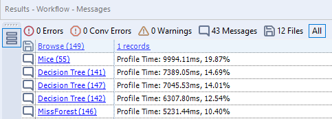
missForest manages to achieve 2X speed faster than MICE!
Summary
In this post, we obtained 2 new assets to tackle missing values. For users who are in the fields require less restrictive methodology, consider implementing in reverse order. First impute with missForest for a quick result, then check with MICE see any improvement area.
Tough crowd? Below are some extra materials and coding block for your further customization. Have fun!
Additional resources:
Multiple Imputation by John Errickson LSA Statistic University of Michican
Using the MissForest Package by Daniel J. Stekhoven
For MICE macro
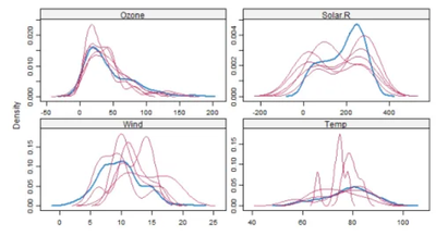
If all variables are numeric, you could uncomment the last part of code to add Density Plot in the Alteryx report:
#Backup report for density plot

AlteryxGraph(5, width=576, height=576)

densityplot(impute)

invisible(dev.off())
For missForest macro:
By default, the macro will use n - 2 cores of your hardware to leave some buffer for background jobs. Feel free to unleash it!
#load package
library(missForest)
library(doParallel)

#define number of cores
numcore = detectCores() - 2

registerDoParallel(cores = numcore)
Editor's note: Updated 2021-03-26 to remove references to MCAR macro which is no longer available.