
 Opening Day
Well it's that time of the year again in the United States. The 162 game marathon MLB season is officially underway. In honor of the opening of another season of America's Pasttime I was working on a post that uses data from the MLB. What I realized was that as I was writing the post, I found that I kept struggling with inconsistent data across different seasons. It was really annoying and finally it hit me: This is what I should be writing about! Why not just dedicate an entire post to normalizing data!
So that's what I've done. In this post we'll be digging into some MLB payroll data. In particular I'm going to show you how you can use normalization techniques to compare seemlingly incomparable data! Sounds like magic? Well it's actually really simple, but I think these little Python scripts will really help you out 🙂
Our Data
The data I'm using is a collection of MLB standings and attendance data from the past 70 years. You can read more about how I collected it in this post
I'm sure a lot of you saw the news last week about feather, the brainchild from Wes McKinney and Hadley Wickham. As both a Python and an R user, I think it's a really compelling idea. It'll be interesting to see how the project progresses over time. Can't wait to see what else they cook up!
In any event, I thought I'd give it a try for this post. I did my data collection using R (comes from a previous post on the MLB), but I wanted to do the analysis in Rodeo. After running my data collection script in R, I sent the output to a .feather file using the feather R package.
<span class="pln">library</span><span class="pun">(</span><span class="pln">feather</span><span class="pun">)</span><span class="pln">
write_feather</span><span class="pun">(</span><span class="pln">standings</span><span class="pun">,</span> <span class="str">"standings.feather"</span><span class="pun">)</span><span class="pln">
write_feather</span><span class="pun">(</span><span class="pln">attendance</span><span class="pun">,</span> <span class="str">"attendance.feather"</span><span class="pun">)</span>
I then read that data back into Python.
<span class="kwd">import</span><span class="pln"> feather
</span><span class="kwd">import</span><span class="pln"> pandas </span><span class="kwd">as</span><span class="pln"> pd
standings </span><span class="pun">=</span><span class="pln"> feather</span><span class="pun">.</span><span class="pln">read_dataframe</span><span class="pun">(</span><span class="str">'./standings.feather'</span><span class="pun">)</span><span class="pln">
attendance </span><span class="pun">=</span><span class="pln"> feather</span><span class="pun">.</span><span class="pln">read_dataframe</span><span class="pun">(</span><span class="str">'./attendance.feather'</span><span class="pun">)</span>
| | 1run | exinn | g | home | inter | l | last_year | lg | luck | pythwl | r | ra | rdiff | rk | road | sos | srs | tm | vlhp | vrhp | vs_teams_above_500 | vs_teams_below_500 | w | wins_losses | year |
|---|
| 0 | 22-19 | 5-3 | 155.0 | 53-24 | None | 56.0 | 1949.0 | AL | 2 | 96-58 | 5.9 | 4.5 | 1.4 | 1 | 45-32 | -0.2 | 1.3 | NYY | 42-25 | 56-31 | 38-28 | 60-28 | 98.0 | 0.636 | 1950 |
|---|
| 1 | 30-16 | 7-4 | 157.0 | 48-29 | None | 63.0 | 1949.0 | NL | 4 | 87-67 | 4.6 | 4.0 | 0.6 | 2 | 43-34 | -0.1 | 0.5 | PHI | 20-17 | 71-46 | 46-42 | 45-21 | 91.0 | 0.591 | 1950 |
|---|
| 2 | 20-20 | 8-4 | 157.0 | 50-30 | None | 59.0 | 1949.0 | AL | 7 | 88-66 | 5.3 | 4.5 | 0.8 | 3 | 45-29 | -0.1 | 0.7 | DET | 37-23 | 58-36 | 32-34 | 63-25 | 95.0 | 0.617 | 1950 |
|---|
| 3 | 23-21 | 5-8 | 155.0 | 48-30 | None | 65.0 | 1949.0 | NL | 1 | 88-66 | 5.5 | 4.7 | 0.8 | 4 | 41-35 | -0.1 | 0.7 | BRO | 35-20 | 54-45 | 48-40 | 41-25 | 89.0 | 0.578 | 1950 |
|---|
| 4 | 21-11 | 4-5 | 154.0 | 55-22 | None | 60.0 | 1949.0 | AL | 0 | 94-60 | 6.7 | 5.2 | 1.4 | 5 | 39-38 | -0.2 | 1.3 | BOS | 31-22 | 63-38 | 29-37 | 65-23 | 94.0 | 0.610 | 1950 |
|---|
| | attend_per_game | attendance | batage | bpf | est_payroll | managers | n_a_ta_s | n_aallstars | n_hof | page | ppf | time | tm | year |
|---|
| 0 | 10708.0 | 535418.0 | 26.5 | 103 | 5571200.0 | Cox | 15 | 1 | 2 | 31.5 | 103 | 2:37 | ATL | 1981 |
|---|
| 1 | 18623.0 | 1024247.0 | 30.2 | 100 | NaN | Weaver | 13 | 3 | 3 | 29.3 | 99 | 2:42 | BAL | 1981 |
|---|
| 2 | 20007.0 | 1060379.0 | 29.2 | 106 | NaN | Houk | 15 | 1 | 4 | 27.9 | 106 | 2:40 | BOS | 1981 |
|---|
| 3 | 26695.0 | 1441545.0 | 30.5 | 99 | 3828834.0 | Fregosi and Mauch | 13 | 4 | 1 | 30.0 | 99 | 2:40 | CAL | 1981 |
|---|
| 4 | 9752.0 | 565637.0 | 28.2 | 104 | NaN | Amalfitano | 14 | 1 | 0 | 28.1 | 106 | 2:42 | CHC | 1981 |
|---|
Wow! Really easy. Great work Wes and Hadley! 🙂
Now that we've got our data, it's time to do some munging.
The Problem
I'm looking to compare payrolls over time. There are a couple of tricky things about this.
First off (and probably most obviously) is that the value of the dollar has changed over the past 70 years. So there will be obvious differences between a payroll from 1970 and a payroll from 2010.
<span class="pln">payrolls </span><span class="pun">=</span><span class="pln"> attendance</span><span class="pun">[[</span><span class="str">'year'</span><span class="pun">,</span> <span class="str">'est_payroll'</span><span class="pun">]].</span><span class="pln">groupby</span><span class="pun">(</span><span class="str">'year'</span><span class="pun">).</span><span class="pln">mean</span><span class="pun">()</span> <span class="pun">/</span> <span class="lit">1000</span><span class="pln">
payrolls</span><span class="pun">[(</span><span class="pln">payrolls</span><span class="pun">.</span><span class="pln">index</span><span class="pun">==</span><span class="lit">1970</span><span class="pun">)</span> <span class="pun">|</span> <span class="pun">(</span><span class="pln">payrolls</span><span class="pun">.</span><span class="pln">index</span><span class="pun">==</span><span class="lit">2010</span><span class="pun">)]</span>
<span class="typ">Out</span><span class="pun">[</span><span class="lit">24</span><span class="pun">]:</span><span class="pln">
 est_payroll </span><span class="pun">(</span><span class="lit">1000s</span><span class="pun">)</span><span class="pln">
year
</span><span class="lit">1970</span> <span class="lit">434.565455</span>
<span class="lit">2010</span> <span class="lit">91916.006567</span>
Yikes! When adjusted for inflation, that $434k becomes $2.5M. Compare that to the actual average payroll in 2010, $92M, and not quite everything seems to be adding up.
That's because the value of baseball players has ALSO been increasing over time. As teams have been able to make more money through TV revenue and other means, ballplayers salaries have gone up...way up! As a result normalizing our data isn't as simple as just adjusting for inflation. Darn!
Brief Aside: While on the subject, a super interesting factoid is the "Bobby Bonilla Mets contract". Despite having been retired for 15 years, the Mets still pay him over $1M per year, thanks to an interesting negotiation and Mets owner Fred Wilpon's involvement in Bernie Madoff's Ponzi scheme. Full story here.

Bobby Bonilla still makes over $1M / year despite not having played baseball since 2001
Basic Normalization
Not to worry! We can still get an apples to apples comparison of payrolls over time. In order to make that comparison, we need our payrolls to be on the same numerical scale.
We're going to use a really simple approach for this. For each year we're going to calculate the mean salary for the league as whole, and then create a derived field which compares a given team's payroll to the mean payroll for the entire league.
Lucky for us, Python and pandas make this super easy to do. Here goes...
<span class="pln">mean_payrolls </span><span class="pun">=</span><span class="pln"> attendance</span><span class="pun">[[</span><span class="str">'year'</span><span class="pun">,</span> <span class="str">'est_payroll'</span><span class="pun">]].</span><span class="pln">groupby</span><span class="pun">(</span><span class="str">'year'</span><span class="pun">).</span><span class="pln">mean</span><span class="pun">().</span><span class="pln">reset_index</span><span class="pun">()</span><span class="pln">
mean_payrolls</span><span class="pun">.</span><span class="pln">columns </span><span class="pun">=</span> <span class="pun">[</span><span class="str">'year'</span><span class="pun">,</span> <span class="str">'league_mean_payroll'</span><span class="pun">]</span><span class="pln">
attendance </span><span class="pun">=</span><span class="pln"> pd</span><span class="pun">.</span><span class="pln">merge</span><span class="pun">(</span><span class="pln">attendance</span><span class="pun">,</span><span class="pln"> mean_payrolls</span><span class="pun">,</span><span class="pln"> on</span><span class="pun">=</span><span class="str">'year'</span><span class="pun">)</span><span class="pln">
attendance</span><span class="pun">[</span><span class="str">'norm_payroll'</span><span class="pun">]</span> <span class="pun">=</span><span class="pln"> attendance</span><span class="pun">.</span><span class="pln">est_payroll </span><span class="pun">/</span><span class="pln"> attendance</span><span class="pun">.</span><span class="pln">league_mean_payroll</span>
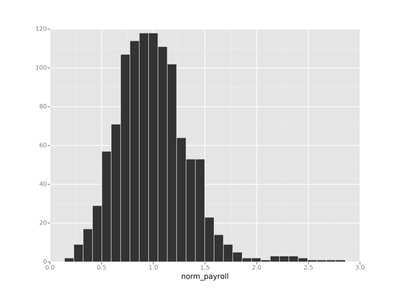
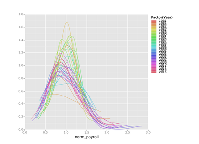
Let's take a look at what our norm_payroll field looks like. Ahh there we go!
Getting the 0 to 1 Value
But what if we wanted to do something a little different? for instance, what if you wanted the norm_payroll to bet a standardized value between 0 and 1 (instead of a uncapped scale as in the previous example)?
This is actually something that's really common. Many machine learning algorithms perform much better using scaled data (support vector machine comes to mind). Again, lucky for us doing this in Python is super easy.
To do this we'll use the same approach as before (as in, normalizing by year) but instead of using the mean, we're going to use the max and min values for each year.
<span class="pln">min_payrolls </span><span class="pun">=</span><span class="pln"> attendance</span><span class="pun">[[</span><span class="str">'year'</span><span class="pun">,</span> <span class="str">'est_payroll'</span><span class="pun">]].</span><span class="pln">groupby</span><span class="pun">(</span><span class="str">'year'</span><span class="pun">).</span><span class="pln">min</span><span class="pun">().</span><span class="pln">reset_index</span><span class="pun">()</span><span class="pln">
min_payrolls</span><span class="pun">.</span><span class="pln">columns </span><span class="pun">=</span> <span class="pun">[</span><span class="str">'year'</span><span class="pun">,</span> <span class="str">'league_min_payroll'</span><span class="pun">]</span><span class="pln">
max_payrolls </span><span class="pun">=</span><span class="pln"> attendance</span><span class="pun">[[</span><span class="str">'year'</span><span class="pun">,</span> <span class="str">'est_payroll'</span><span class="pun">]].</span><span class="pln">groupby</span><span class="pun">(</span><span class="str">'year'</span><span class="pun">).</span><span class="pln">max</span><span class="pun">().</span><span class="pln">reset_index</span><span class="pun">()</span><span class="pln">
max_payrolls</span><span class="pun">.</span><span class="pln">columns </span><span class="pun">=</span> <span class="pun">[</span><span class="str">'year'</span><span class="pun">,</span> <span class="str">'league_max_payroll'</span><span class="pun">]</span><span class="pln">
attendance </span><span class="pun">=</span><span class="pln"> pd</span><span class="pun">.</span><span class="pln">merge</span><span class="pun">(</span><span class="pln">attendance</span><span class="pun">,</span><span class="pln"> min_payrolls</span><span class="pun">,</span><span class="pln"> on</span><span class="pun">=</span><span class="str">'year'</span><span class="pun">)</span><span class="pln">
attendance </span><span class="pun">=</span><span class="pln"> pd</span><span class="pun">.</span><span class="pln">merge</span><span class="pun">(</span><span class="pln">attendance</span><span class="pun">,</span><span class="pln"> max_payrolls</span><span class="pun">,</span><span class="pln"> on</span><span class="pun">=</span><span class="str">'year'</span><span class="pun">)</span><span class="pln">
attendance</span><span class="pun">[</span><span class="str">'norm_payroll_0_1'</span><span class="pun">]</span> <span class="pun">=</span> <span class="pun">(</span><span class="pln">attendance</span><span class="pun">.</span><span class="pln">est_payroll </span><span class="pun">-</span><span class="pln"> attendance</span><span class="pun">.</span><span class="pln">league_min_payroll</span><span class="pun">)</span> <span class="pun">/</span> <span class="pun">(</span><span class="pln">attendance</span><span class="pun">.</span><span class="pln">league_max_payroll </span><span class="pun">-</span><span class="pln"> attendance</span><span class="pun">.</span><span class="pln">league_min_payroll</span><span class="pun">)</span>
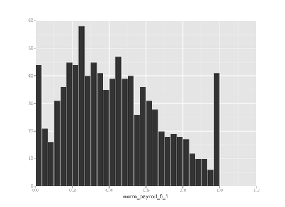
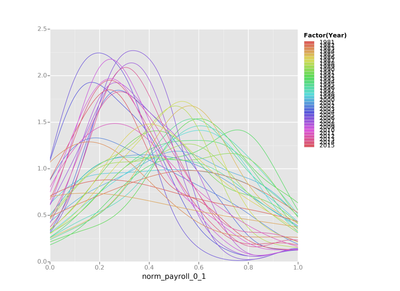
As you can see things actually look a bit different than they did using the first method. Keep this in mind: Your normalization strategy can impact your results! Please don't forget this!
There You Have It
There are lots more ways to normalize your data (really whatever strategy you can think of!). These are just 2 ways that work a lot of the time and can be nice starting points. By no means is this the end all be all of data normalization (there are many books on the subject), but hopefully this gives you a quick intro to this very important topic.
Till next time--enjoy the season, the normalization techniques and the new feather file format!
Still around, huh? Looking for other resources on data normalization? Look no further: