Alteryx Designer Desktop Discussions
Find answers, ask questions, and share expertise about Alteryx Designer Desktop and Intelligence Suite.- Community
- :
- Community
- :
- Participate
- :
- Discussions
- :
- Designer Desktop
- :
- Re: Performing vlookup with Combining the data wit...
Performing vlookup with Combining the data within cell
- Subscribe to RSS Feed
- Mark Topic as New
- Mark Topic as Read
- Float this Topic for Current User
- Bookmark
- Subscribe
- Mute
- Printer Friendly Page
- Mark as New
- Bookmark
- Subscribe
- Mute
- Subscribe to RSS Feed
- Permalink
- Notify Moderator
I have two files which would need Vlookup to be performed to update the fields for other, the twist is i need the information of the columns to be joined/combined while performing vlookup. (Col. B and F) highlighted in Yellow.
Unique number is Asset #
I attached the an example of files. First one is the Old, and second Import 2 - update is recent one with updated information.
Solved! Go to Solution.
- Labels:
-
Join
- Mark as New
- Bookmark
- Subscribe
- Mute
- Subscribe to RSS Feed
- Permalink
- Notify Moderator
@nirkisna65
I am sorry but I did not quite get what your desire.
But check this and it is just simple.
- Mark as New
- Bookmark
- Subscribe
- Mute
- Subscribe to RSS Feed
- Permalink
- Notify Moderator
Sorry, let me rephrase it. I want to combine the data of both the columns in to the updated export. For Eg: Spreadsheet, Import - Old, Col. B4 has "XYZ" where as 2nd spreadsheet Import 2 updated - report, Col. B4 has "Zee"... I want work flow result to give Col. B4 as "XYZ. Zee"
same to be performed for Col. F.
I could open the workflow share earlier.
Thanks for your help @Qiu
- Mark as New
- Bookmark
- Subscribe
- Mute
- Subscribe to RSS Feed
- Permalink
- Notify Moderator
Hi @nirkisna65 ,
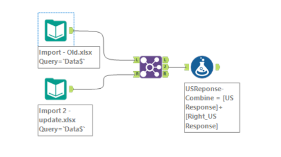
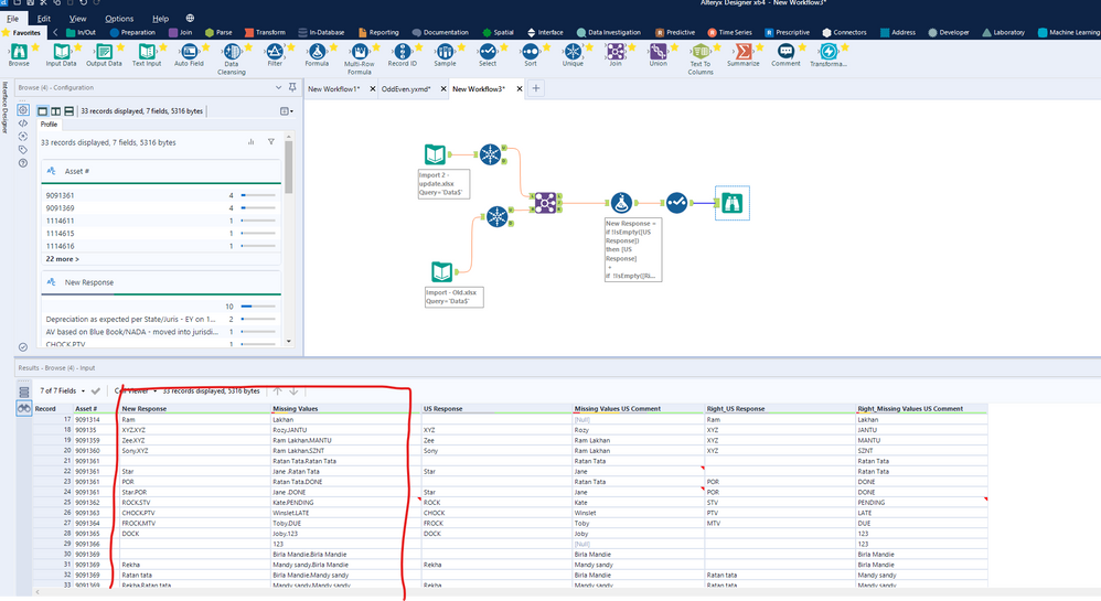
I think you just need to join the data and then concatenate some of the columns?
Please see an image and an example (please add your files to the workflow) attached.Please note that there are some duplicates due to duplicates in the Excel itself. This can be handled of course. You may also need some formatting improvement on the formulas (e.g. only concatenate the values if they differ?), but wasn't sure if that's needed.
Formulas are both following this style:
if !IsEmpty([US Response])
then [US Response]
+
if !IsEmpty([Right_US Response])
then '.'+[Right_US Response]
else ''
endif
else
[Right_US Response]
endif
Regards,
Tom
- Mark as New
- Bookmark
- Subscribe
- Mute
- Subscribe to RSS Feed
- Permalink
- Notify Moderator
Thank you! @TomWelgemoed
- Mark as New
- Bookmark
- Subscribe
- Mute
- Subscribe to RSS Feed
- Permalink
- Notify Moderator
Happy that helped!
Don't forget to watch out for duplicates in the 2 data sets - but hopefully this gets you on your way.
- Mark as New
- Bookmark
- Subscribe
- Mute
- Subscribe to RSS Feed
- Permalink
- Notify Moderator
I have a unique ID as asset number in both the data, do I have change the "Unique" tool for it?
- Mark as New
- Bookmark
- Subscribe
- Mute
- Subscribe to RSS Feed
- Permalink
- Notify Moderator
Hi @nirkisna65 ,
We're already joining on the Asset ID (think that's your only unique number?), but that doesn't appear to be Unique.So you have duplicates in the source data (rightly or wrongly). Try to see if there is not another field that can uniquely identify each row?
Regards,
Tom
- Mark as New
- Bookmark
- Subscribe
- Mute
- Subscribe to RSS Feed
- Permalink
- Notify Moderator
@TomWelgemoed @Qiu Thank you this is awesome. I have another query if you could help, I need to run the conditional formatting to the attached example sheet " Conditional formatting".
I want Color GREEN Col A, B and C if the Col. E is Y, and color RED if Col E. is N and leave out the blank in Col. E as is.
Also, the font of the whole worksheet should be Arial 8 as standard
Could you please help, I tried the rendered tool was not successful to export.
- Mark as New
- Bookmark
- Subscribe
- Mute
- Subscribe to RSS Feed
- Permalink
- Notify Moderator
Hi @nirkisna65,
Thanks for the question, I don't play with the report settings often so it forced me to do that a bit.
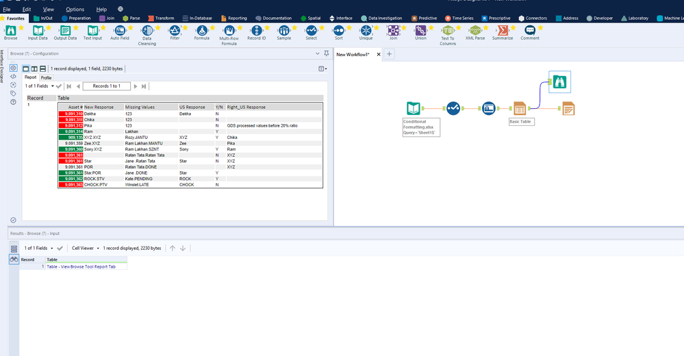
See the image below (I'm a bit busy, so only did it for column A), but you can easily apply the rule to each column where you want it. The key is to use the table tool and then select each field and click the "Column Rules" button on the right (Another image attached, together with the workflow). Then you simply select how you want the rule to go (like in Excel) and how you want to format the column. Also, there is a "Default Table Settings" in this tool, where you can set the font & size. After this you can render the output to Excel.
Hope that helps!
Best,
Tom
-
Academy
6 -
ADAPT
2 -
Adobe
203 -
Advent of Code
3 -
Alias Manager
77 -
Alteryx Copilot
24 -
Alteryx Designer
7 -
Alteryx Editions
89 -
Alteryx Practice
20 -
Amazon S3
149 -
AMP Engine
250 -
Announcement
1 -
API
1,206 -
App Builder
116 -
Apps
1,358 -
Assets | Wealth Management
1 -
Basic Creator
14 -
Batch Macro
1,551 -
Behavior Analysis
245 -
Best Practices
2,690 -
Bug
719 -
Bugs & Issues
1 -
Calgary
67 -
CASS
53 -
Chained App
267 -
Common Use Cases
3,819 -
Community
26 -
Computer Vision
85 -
Connectors
1,424 -
Conversation Starter
3 -
COVID-19
1 -
Custom Formula Function
1 -
Custom Tools
1,934 -
Data
1 -
Data Challenge
10 -
Data Investigation
3,484 -
Data Science
3 -
Database Connection
2,215 -
Datasets
5,215 -
Date Time
3,226 -
Demographic Analysis
186 -
Designer Cloud
737 -
Developer
4,359 -
Developer Tools
3,525 -
Documentation
526 -
Download
1,036 -
Dynamic Processing
2,933 -
Email
926 -
Engine
145 -
Enterprise (Edition)
1 -
Error Message
2,253 -
Events
196 -
Expression
1,867 -
Financial Services
1 -
Full Creator
2 -
Fun
2 -
Fuzzy Match
711 -
Gallery
666 -
GenAI Tools
2 -
General
2 -
Google Analytics
155 -
Help
4,703 -
In Database
965 -
Input
4,288 -
Installation
359 -
Interface Tools
1,898 -
Iterative Macro
1,090 -
Join
1,955 -
Licensing
251 -
Location Optimizer
60 -
Machine Learning
259 -
Macros
2,857 -
Marketo
12 -
Marketplace
23 -
MongoDB
82 -
Off-Topic
5 -
Optimization
750 -
Output
5,241 -
Parse
2,325 -
Power BI
227 -
Predictive Analysis
936 -
Preparation
5,159 -
Prescriptive Analytics
205 -
Professional (Edition)
4 -
Publish
257 -
Python
851 -
Qlik
39 -
Question
1 -
Questions
2 -
R Tool
476 -
Regex
2,339 -
Reporting
2,428 -
Resource
1 -
Run Command
572 -
Salesforce
276 -
Scheduler
410 -
Search Feedback
3 -
Server
628 -
Settings
932 -
Setup & Configuration
3 -
Sharepoint
624 -
Spatial Analysis
599 -
Starter (Edition)
1 -
Tableau
512 -
Tax & Audit
1 -
Text Mining
468 -
Thursday Thought
4 -
Time Series
430 -
Tips and Tricks
4,182 -
Topic of Interest
1,124 -
Transformation
3,720 -
Twitter
23 -
Udacity
84 -
Updates
1 -
Viewer
3 -
Workflow
9,960
- « Previous
- Next »


