At a high-level, forecasting techniques can be broken down into three main categories:
- Historical Average with Sliding Windows
- Examples: Seasonal Decomposition, Exponential Smoothing (ETS)
- Pros: Simplicity: any tool can integrate like Excel & Tableau;
- Cons: Laggardly reaction to changes & overly responsive with outliers, only works with simple structure
- Linear Models
- Examples: ARIMA, VAR(Good for multiple time series)
- Pros: Works with consistent variation, such as established seasonality trends
- Cons: Proper assumption on stationarity and homoscedasticity (statistics term for consistent variance/error). Careful predictor selection to prevent multicollinearity (statistics term when predictors are linearly correlated).
- Non-Linear Models
- Examples: Prophet, GARCH (generalized autoregressive conditional heteroskedasticity), Deep Learning
- Pros: Discovering non-linear relationship & data drift in your data. Example: stocks, holidays, etc.
- Cons: Requires a large amount of data, setup, and maintenance. Prone to overfitting.
Christmas Sales are Coming
Prophet is the open-source package developed by Facebook, belonging to the non-linear model subset. However, it uses relatively much less data and configuration to build an accurate forecast model. In fact, the package became popular because of its easiness and robustness to handle missing value & data shifts.
To start with, download the workflow including the Prophet tool here. We will use one of the Kaggle competitions, Rossmann Store Sales, for our modeling. Why did we choose this? Because it involves CHRISTMAS!!!

Okay, to be more specific: it involves a holiday parameter. To understand better, we have to know the core of Prophet:
Prophet is an additive model with three main components: Seasonality, Changepoint & Holidays
- Seasonality: Decompose data into Trend, Yearly/Weekly/Daily Seasonality & Noise. Similar to Time Series Plot.
- Changepoint: Potential changepoints are placed with the rating scale to detect the shift in trend automatically.
- Holiday: A pre-defined list to capture more than 63 countries’ holidays in the model. User-defined list is possible.
Let’s put theory into practice.
(Note: make sure you have internet access when open the workflow for package installation.)
Summary
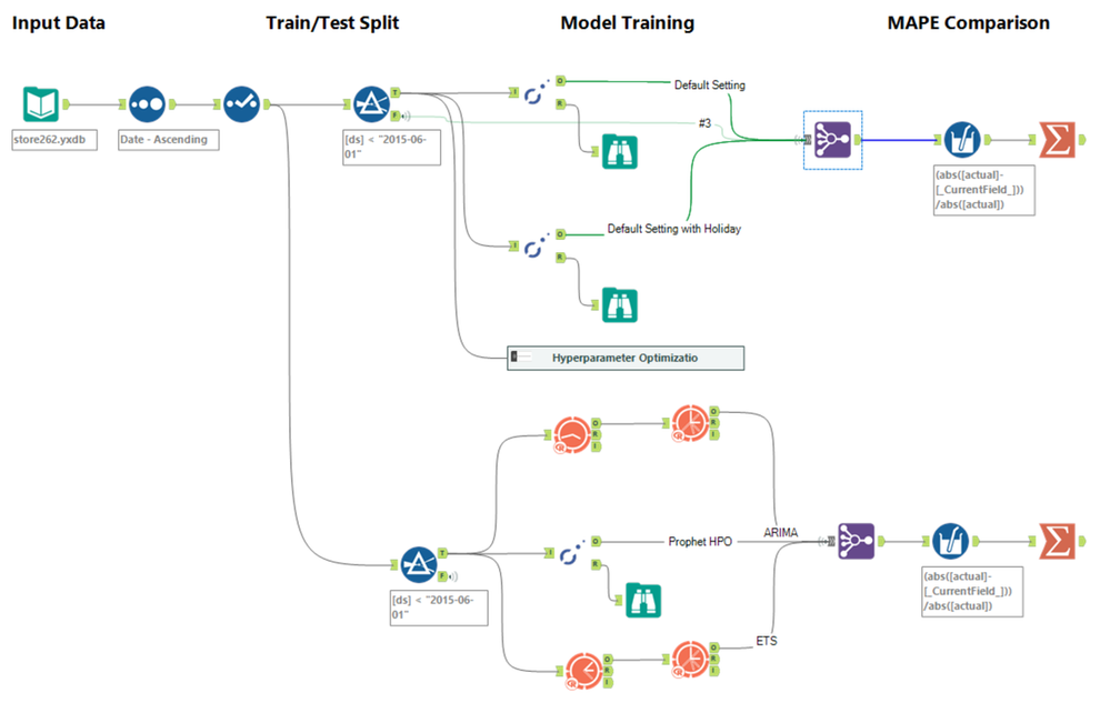
First, we filter the store sales history into training and testing set per Kaggle instruction. Instead of six weeks ahead, we go further and set to eight weeks, which in total 61 days. We then run Prophet tools with three settings together with ARIMA & ETS and calculate the mean absolute percentage error (MAPE) based on the actual data and forecasted result.
Basic
I Data Input
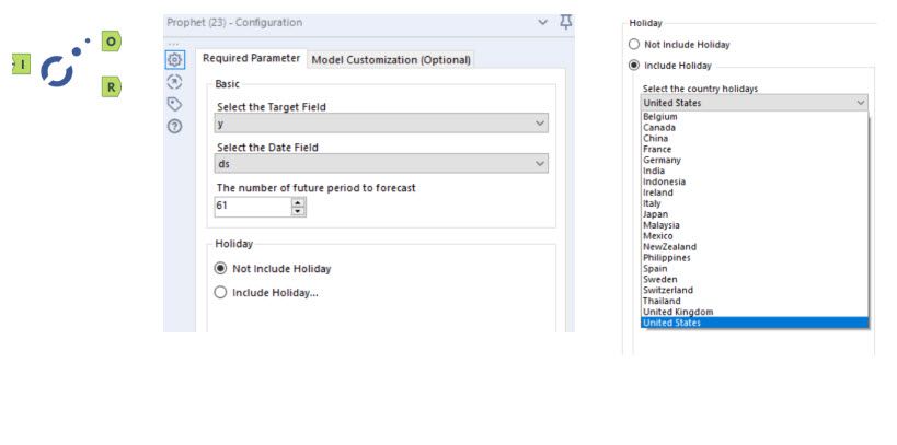
At a minimum, Prophet only requires two columns: Date Time & Target. Specify how many periods to forecast: 61 in this case. Prophet will analyze the whole time series and build the model accordingly.
In the same window, you could also include Holiday as a parameter. If you check that box, you will find a collection of countries to pick. Here we will choose Germany since it’s the company base. Feel free to try out others and let us know!
O Forecast output
Same as the TS Forecast tool, Prophet outputs forecast values and its lower & upper confidence bound. It also provides a forecasted trend for analysts to further engineer.

R Report Output
Components Plot & Changepoint Chart are provided to understand the model effect.
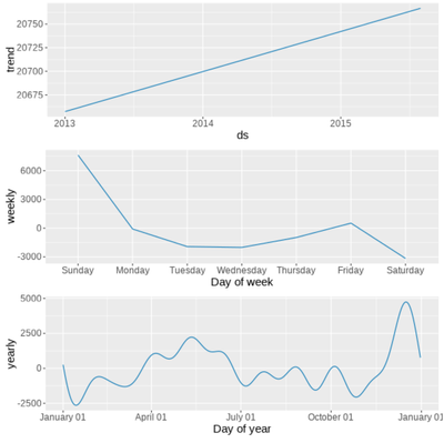
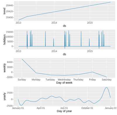
The components plot visualizes the trend, daily/weekly/yearly seasonality and the Holiday effect.
Below are the component plots from the first two Prophet tools. By adding the Germany public holidays on the right, we could observe there are spikes in April (Easter), June/July (Summer), Oct (German Unity or Oktoberfest?), Dec (Christmas!). These spikes indicate the high degree of holiday effect on the drug store sales every year. Furthermore, the trends with the holiday elements show more layers while the yearly seasonality is less fluctuated.
First Comparison
Check out the first Summarize tool. You will see the Prophet model with holiday parameter performs better than the one without. A 0.04 percent accuracy improvement. Not bad considered it’s an out of the box feature! Let’s fine-tune the model further.

Advanced
Hyperparameter Optimization
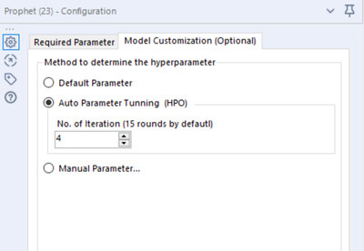
After building your first two models, it’s time to tune the hyperparameters. Switch to the Model Customization Tab and check the Auto Parameter Tuning (HPO) option.
To make this tool more automatic, a Bayesian Optimization function is added to tune the following hyperparameters:
- Number of Changepoint: Number of potential changepoints to include. Selected automatically if not supplied.
- Changepoint Scale: Flexibility of the changepoint. Large values will allow many changepoints; small values limit it.
- Seasonality scale: Strength of the seasonality model. Larger values allow larger fluctuations, smaller values dampen it
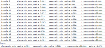
Too many things to tune? No worries. Instead of manually tuning it one by one, here you just need to key in the number of iterations and sit back. The model will start hunting for the best hyperparameters.
Within a few minutes, the result is out.

Manual Parameters
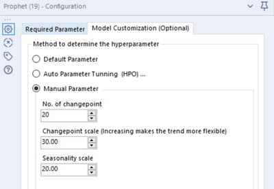
After running the auto parameter options, we found the best parameter set. Running the HPO option every time will incur computation costs. Instead, we will take the numbers and put them in the Manual Parameter option. Here our final Prophet HPO model is produced.
To look at the model difference, we will check out the R report one more time.
The changepoint chart visualize at which point the time series abruptly changed.
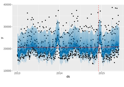
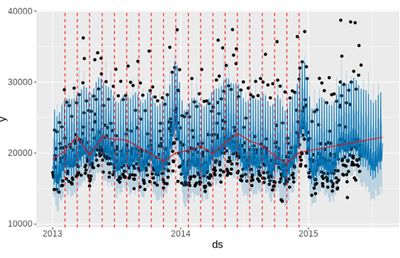
With the new set of parameters, the model successfully uncovers the non-linear trends across three years, which previously can only see a slight upward trend. How does this finalized Prophet HPO model perform? Let’s bring in ARIMA & ETS in order to make the comparison.
Second Comparison
In the second summarize tool, we can see the Prophet HPO model’s accuracy further improved. It is also stunning to see the ARIMA & ETS MAPE is much higher than the Prophet model. An ensemble model between ETS & Prophet can be considered for the next step.

End! And?
That’s all for now! In this post, we learned some fundamental blocks on forecasting techniques. We also introduced a new hot forecasting package: Prophet, including its key components and auto-tuning its hyper-parameters. Once you are ready, feel free to enrich the model with other techniques. e.g., Add external regressors, edit custom dates like promotions, set up saturating maximum for logistic growth, etc.
Additional resources:
For users who are interested to modify the optimization search range & solver at the backend, feel free to open the macro and modify the code inside. Here, the key parameters are highlighted in magenta. Have Fun!
#define hyper search parameter
rand_search_grid = data.frame(
changepoint_prior_scale = sort(runif(10, 0.01, 20)),
seasonality_prior_scale = c(sort(sample(c(runif(5, 0.01, 0.05), runif(5, 1, 20)), 5, replace = F)),
sort(sample(c(runif(5, 0.01, 0.05), runif(5, 1, 20)), 5, replace = F))),
n_changepoints = sample(5:50, 10, replace = F)
...
...
...
ba_search = BayesianOptimization(prophet_fit_bayes,
                                    bounds = bayesian_search_bounds,
                                    init_grid_dt = rand_search_grid,
                                    init_points = 1,
                                    n_iter = %Question.iteration.var%,
 acq = 'ucb',
 kappa = 1,
 eps = 0,
                                    verbose = TRUE)