Tool Mastery
Explore a diverse compilation of articles that take an in-depth look at Designer tools.- Community
- :
- Community
- :
- Learn
- :
- Academy
- :
- Tool Mastery
- :
- Tool Mastery | K-Centroids Cluster Analysis
Tool Mastery | K-Centroids Cluster Analysis
- Subscribe to RSS Feed
- Mark as New
- Mark as Read
- Bookmark
- Subscribe
- Printer Friendly Page
- Notify Moderator
09-24-2018 06:30 AM - edited 08-03-2021 03:43 PM

Cluster analysis has a wide variety of use cases, including harnessing spatial data for grouping stores by location, performing customer segmentation or even insurance fraud detection. Clustering analysis groups individual observations in a way that each group (cluster) contains data that are more similar to one another than the data in other groups. Included with the Predictive Tools installation, the K-Centroids Cluster Analysis Toolallows you to perform cluster analysis on a data set with the option of using three different algorithms:K-Means, K-Medians,andNeural Gas.
One popular use case for cluster analysis is Market Segmentation, which is the process of dividing a large customer base or market into smaller groups of consumers, based on shared characteristics. Cluster analysiswill group potential customers based on shared traits (e.g., age, gender, interests), which can allow a business to focus on sending marketing to the groups with this highest potential, or even create more personalized marketing strategies.
You can think of cluster analysis as the process of creating groups based on where points are plotted in an n-dimensional scatter plot. Generally speaking, the goal is to minimize the distance between points within the same cluster, while also maximizing the distance between cluster groups. Because this type of analysis is based on numeric distance, all of the variables that are being used for clustering need to be continuous. Clustering is an unsupervised classification method, which means you do not provide the target groups for analysis.
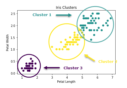
Because n-dimensions can be difficult to imagine, especially when n is more than 3 (which is the number of dimensions we are used to dealing with) I have included a plot of a 2-dimensional example, clustering the Iris data set based on Petal Length (x-axis) and Petal Width (y-axis).
As you can see, observations (records) with similar traits (variable values) are grouped together and labeled as belonging to the same cluster.
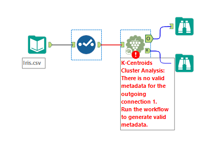
The configuration of the K-Centroids Cluster Analysis Tool is straight-forward. However, before even configuring you might see the following error after connecting the input of the K-Centroids clustering tool to data:
No need to worry, this is a metadata error and will be resolved as soon as the workflow is run.
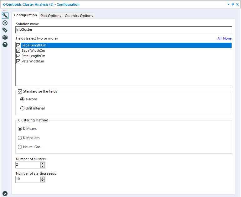
The Configuration Tab for the tool displays all of the options related to the algorithm itself.
The first Configuration Option is the Solution Name. This is the name you want to give to your clustering solution. You can name your clustering solution anything you want, as long as it starts with a letter, and only contains letters, numbers, and the special characters period (".") or underscore ("_").
The next configuration options is Fields. This is a check-box list of the fields that you would like to be considered in your cluster analysis. You will notice that only numeric field types populate in this list. This is because cluster analysis by nature can only be performed on continuous variables. Select the combination of features that you would like your cluster groups to be created from by checking and unchecking the associated boxes. As indicated, you must select two or more variables for cluster analysis.
Once you have your combination of clustering variables selected, you can choose if you’d like to Standardize the fields. Standardization of fields in Cluster Analysis is a frequent practice because of the impact distance between variable values has on the clustering solution. In this tool, your options for standardizing are either to do so with z-score or unit interval standardization. If you would like to read more, please see the Community article: Standardization in Cluster Analysis.
Next, you can select a clustering method. The K-Centroids Cluster Analysis Tool uses the underlying R package flexclustto implement the three clustering algorithm options: K-Means, K-Medians, and Neural Gas. Each of these algorithms approaches the task of dividing data into groups based on distance differently.
K-means partitions the observations in a dataset into any number of clusters (specified in the next step in configuration) by assigning the observation to the cluster with the nearest mean using Euclidian distance.This method effectively partitions the data space into Voronoi cells. The algorithm is implemented iteratively by first randomly selecting n number of points (n being your target number of clusters) as starter centroids, grouping all of the points around these centroids, and recalculating the centroid based on the mean values of each group. This process is repeated until the points become stable (reaching convergence).
K-medians is a variation of k-means, which uses the median to determine the centroid of each cluster, instead of the mean. The median is computed in each dimension (for each variable) with aManhattan distanceformula (think of walking or city-block distance, where you have to follow sidewalk paths). This method is more reliable for discrete variables or even binary data sets.
You can read more about the implementation of both of these algorithms in the flexclust package in the paper:A Toolbox for K-Centroids Cluster Analysis by Friedrich Leisch.
Like K-Means, Neural Gas uses Euclidean distance. However, the location of the centroid of the cluster is a weighted average of all of the data points, with the points assigned to the cluster receiving the greatest weight. The weights for each point become less and less based on the distance rank of the classes. The Neural Gas algorithm implemented in this tool can be read about in the paper “Neural-Gas” Network for Vector Quantization and its Application to Time-Series Predictionby Thomas Martinetz et al.
Your algorithm selection will depend on your data and use case. For help getting started with selecting the appropriate algorithm, check out this chapter on Cluster Analysis from Introduction to Data Mining, or these two Stack Exchange threads from the Cross Validated forum, here and here.
The last two options in the configuration tab are the Number of clusters and the Number of starting seeds.
The number of clusters argument sets the number of target clusters that will be created. If you are hoping to create two groups from your data, you would set this value to 2, for three groups, 3, and so on. If you are not sure what number of clusters is appropriate for your data, consider using the K-Centroids Diagnostics Tool.
The number of starting seeds sets the number of repetitions (nrep, in the R function) argument, which repeats the entire solution building process the specified number of times, and keeps only the best solution. This is a necessary argumentbecause of the random nature of how the clustering algorithms are initiated. The first step is randomly creating points as initial centroids. The final solution can be impacted by where these initial points are created. When using multiple starting seeds, the best solution from all iterations is kept. This is a way of ensuring more consistent clustering solutions. A higher number of starting seeds will help ensure the best possible solution is found; however, higher values will increase the tool’s processing time.
The Plot Options tab of the tool allows you to set Options to Plot Points, Plot Centroids, neither or both. You can also constrain the number of dimensions displayed in your plot. By default, The highest number of dimensions to include in the biplots is set to 2. This is because it is difficult to visually display more than 2-dimensions in a flat plot.
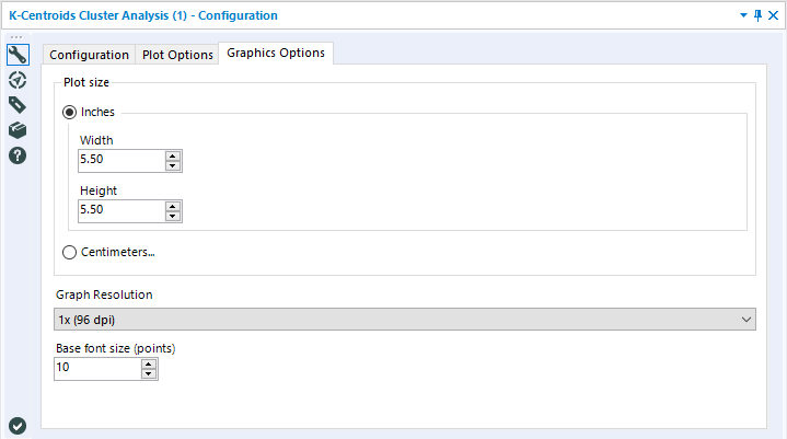
The Graphic Options tab simply lets you configure the graphic components of the plot output with the R anchor. You can specify the size of your plot in inches or centimeters, as well as the Graph Resolution (in dots per inch) and the base font size (in points).
Outputs
Once your tool’s configuration is set, you can run your workflow and see your outputs! There are two output anchors for the K-Centroids Cluster Analysis Tool, an O anchor and an R anchor. The O anchor, as with most predictive tools, is the Model Object. This can be used as an input to the Append Clusters Tool, which allows you to assign the groups to your actual data set.
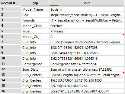
In addition to the Model Object itself, this output includes the call, which is the R code used to generate the model, the Formula itself, the model class, which should always be flexclust (this is the R package used), the Model Object, the information about each of the clusters, separated by pipes (you can think of rows 7-10 as a table, where row 7 contains the headers for each column, and 8, 9, and 10 are each cluster. The number of rows will depend on the number of clusters created). Convergence describes how many iterations were run before the model began to produce consistent clusters. The Sum of Distances can be thought of as an overall model metric. Cluster Centers (rows 13-16) is another table which describes the centroid values for each variable for each cluster. This information can all be parsed out and used as data with a combination of data preparation tools.
The R anchor is a report on the clustering solution.
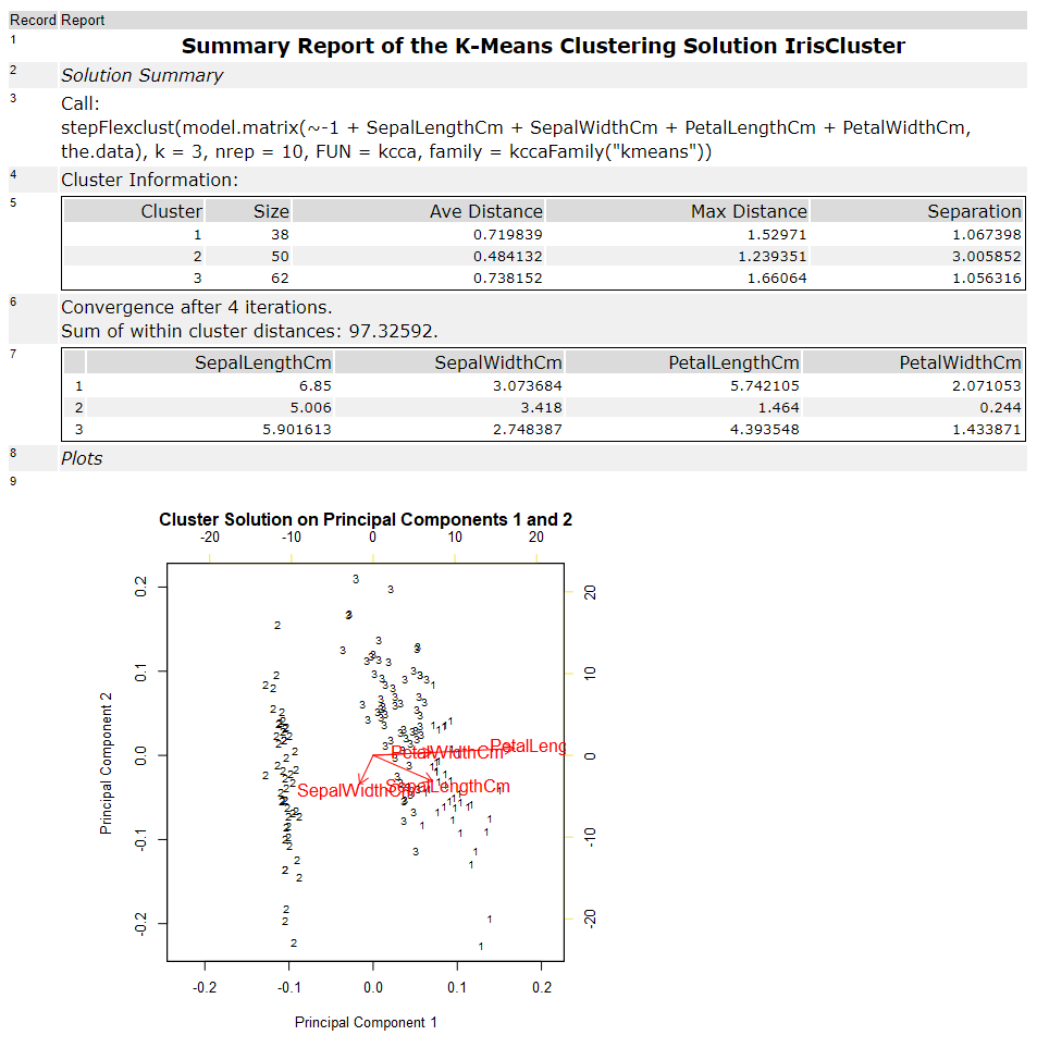
Some of the information included in the O output is also included in the report and formatted so it is more digestible. The Cluster Information (5) and Cluster Centroids (7) are both in legible tables. The Sum of within-cluster distances and convergence, as well as the call, are all in the report. In addition to this information, the Report output also includes a plotted illustration.
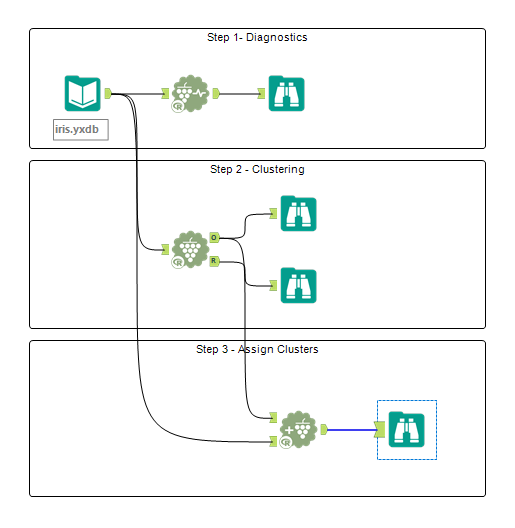
Typically, the K-Centroids Cluster Analysis tool will be used in conjunction with the K-Centroids Diagnostic Tool, and the Append Cluster Tool. The K-Centroids Diagnostics Tool provides information to assist in determining how many clusters to specify, and the Append Cluster Tool functions like a Score Tool, attaching the assigned cluster number to each of your data points.
Used in concert, these three tools can get you through any of your clustering needs!
By now, you should have expert-level proficiency with the K-Centroids Clustering Tool! If you can think of a use case we left out, feel free to use the comments section below! Consider yourself a Tool Master already? Let us know atcommunity@alteryx.comif you’d like your creative tool uses to be featured in the Tool Mastery Series.
Stay tuned with our latest posts every#ToolTuesdayby following@alteryxon Twitter! If you want to master all the Designer tools, considersubscribingfor email notifications.
- Mark as Read
- Mark as New
- Bookmark
- Permalink
- Notify Moderator
I've been doing some clustering and I understand in the Summary Report how to manually calculate the Ave Distance and Max Distance. However, I have not been able to figure out how the Separation is calculated. I'm not necessarily looking for what it means, I want to know how it's calculated. If you or anyone else can answer that I'd greatly appreciate it!
- Mark as Read
- Mark as New
- Bookmark
- Permalink
- Notify Moderator
Nevermind, I figured it out!
- Mark as Read
- Mark as New
- Bookmark
- Permalink
- Notify Moderator
I am actually still looking for more information on the summary report. The things @h_kee mentioned would be helpful including how to calculate average and maximum distance and separation. I would also like to learn more about how to interpret the results. Lastly, I am still unsure what exactly record 7 means and how to interpret that in the R anchor output.
- Mark as Read
- Mark as New
- Bookmark
- Permalink
- Notify Moderator
Hi @BarnesK,
So I figured out how to calculate each of those measures on the summary report (Ave Distance, Max Distance, and Separation). Max Distance and Separation aren't calculations, which I knew for Max Distance but figured out through a lot of trial/error for Separation. I hope my explanation below helps.
An observation belongs to a cluster where it's Euclidean distance is the closest to that cluster. Each observation will be some distance from each cluster but will belong to the cluster with the smallest distance.
In the example in this thread, there are 150 observations, 38 in cluster 1, 50 in cluster 2, and 62 in cluster 3. Using cluster 1 as an example, those 38 observations have an average Euclidean distance of 0.719839 from the cluster 1's mean.
In case you need a refresher on Euclidean distance, i'll give you an example as opposed to the complicated-looking formula!
Observation 1 (these are made up numbers)
Sepal Length - 7
Sepal Width - 3
Petal Length - 6
Petal Width - 2
Record 7 gives you the means for each of those attributes for each cluster. So basically, to get the Euclidean distance from each cluster for Observation 1, you'll need to square each of the differences and then take the square root of the sums.
Ex) Cluster 1 (7-6.85)^2 + (3-3.073684)^2 + (6-5.742105)^2 + (2-2.071053)^2 = 0.315417 Square root of the sum - Euclidean distance
Cluster 2 (7-5.006)^2 + (3-3.418)^2 + (6-1.464)^2 + (2-0.244)^2 = 5.27348 Square root of the sum - Euclidean distance
Cluster 3 (7-5.901613)^2 + (3-2.748387)^2 + (6-4.393548)^2 + (2-1.433871)^2 = 2.042291 Square root of the sum - Euclidean distance
--> This gives you the Euclidean distance from each cluster for observation 1. So since the smallest distance is 0.315417, this observation would belong in cluster 1. So you'll have to repeat that for all 150 observations to get each observations' Euclidean distance from each cluster. Luckily you can get that output from alteryx.
So, going back to the beginning of this example, the 0.719839 is the average Euclidean distance of the observations that belong to cluster 1.
The Max Distance is simply the largest distance of the values that belong to a cluster. So out of the 38 observations for cluster 1, the largest Euclidean distance is 1.52971
The Separation took me longer than it should to figure out and I hope my explanation makes sense. For those 38 observations, each of their Euclidean distances are the closest to cluster 1. In the example I used, observation 1 had a distance of 5.27348 from cluster 2 and 2.042291 from cluster 3. The other observations in this cluster would also have some distance from cluster 2 and cluster 3. The separation is simply the smallest Euclidean distance of the 38 observations from either cluster 2 or cluster 3. So essentially one of the 38 observations for cluster 1 had a distance of 1.067398 from either cluster 2 or 3.
Let me know if that helps, I prefer examples and laymen's terms when explaining these concepts so I hope it made sense.
- Mark as Read
- Mark as New
- Bookmark
- Permalink
- Notify Moderator
Hi @h_kee,
Thanks for the excellent write-up. Is it fair to say that cluster 2 is the cluster that we can rely on based on the "separation", since it has the largest distance from others
- Mark as Read
- Mark as New
- Bookmark
- Permalink
- Notify Moderator
Thank you for the excellent write-up. This is perfect after watching the interactive video, to consolidate the knowledge.
-
2018.3
1 -
API
2 -
Apps
7 -
AWS
1 -
Configuration
3 -
Connector
3 -
Data Investigation
10 -
Database Connection
2 -
Date Time
4 -
Designer
1 -
Desktop Automation
1 -
Developer
8 -
Documentation
3 -
Dynamic Processing
10 -
Error
4 -
Expression
6 -
FTP
1 -
Fuzzy Match
1 -
In-DB
1 -
Input
6 -
Interface
7 -
Join
7 -
Licensing
2 -
Macros
7 -
Output
2 -
Parse
3 -
Predictive
16 -
Preparation
16 -
Prescriptive
1 -
Python
1 -
R
2 -
Regex
1 -
Reporting
12 -
Run Command
1 -
Spatial
6 -
Tips + Tricks
2 -
Tool Mastery
99 -
Transformation
6 -
Visualytics
1
- « Previous
- Next »
