Tool Mastery
Explore a diverse compilation of articles that take an in-depth look at Designer tools.- Community
- :
- Community
- :
- Learn
- :
- Academy
- :
- Tool Mastery
- :
- Tool Mastery | Boosted Model
Tool Mastery | Boosted Model
- Subscribe to RSS Feed
- Mark as New
- Mark as Read
- Bookmark
- Subscribe
- Printer Friendly Page
- Notify Moderator
05-22-2019 11:51 AM - edited 08-03-2021 11:04 AM

This article is part of the Tool Mastery Series, a compilation of Knowledge Base contributions to introduce diverse working examples for Designer Tools. Here we’ll delve into uses of the Boosted Model Tool on our way to mastering the Alteryx Designer:
The Boosted Model tool in Alteryx is a powerful predictive analytics tool. It is one of the more complex tools in the tool chest, but in difficult use cases, it proves to be very valuable. This article will explain what boosting is and provide step-by-step instructions on how to incorporate this technique in a workflow, illustrated with a credit card fraud detection use case. In the Predictive Set of Tools in Alteryx, the very first one on the left is the Boosted Model. The icon for the tool has an upward arrow and what looks like an upright spring.
What is the Boosted Model?
The Boosted Model relies on the machine learning technique known as boosting, in which small decision trees (“stumps”) are serially chain-linked together. Each successive tree in the chain is optimized to better predict the errored records from the previous link. How to better-predict those previous errors is what distinguishes each boosting algorithm. One of the strongest and most proven algorithms is the Gradient Boosting Machine (aka “GBM”). Both R and Python have GBM packages; the Alteryx Boosted Model Tool uses the R implementation.
The Gradient Boosting Machine was invented by Jerome Friedman two decades ago while he was a Statistics Professor at Stanford University. You can download his paper here. A Gradient Boosting Machine is one that uses gradient descent as the method of zeroing in on the errors from the previous tree in the chain.
Boosting – especially gradient boosting – is very popular because of how well it works. New alternative versions of GBM are available in R and Python. The most popular are XGBoost developed in 2014, CatBoost developed in 2017, and Light GBM developed in 2017.
Since the Gradient Boosting Machine uses gradient descent, it needs to have a learning rate configured for it, like other gradient descent algorithms. For GBM, the learning rate is called the “shrinkage factor”.
Gradient boosting (as well as other boosting algorithms) is resistant to overfitting which is basically when an algorithm learns too much about the specifics of the data records it initially learns on, thereby failing to generalize to new, previously unseen, data at prediction time. This is a common problem with many algorithms, but not so much with gradient boosting.
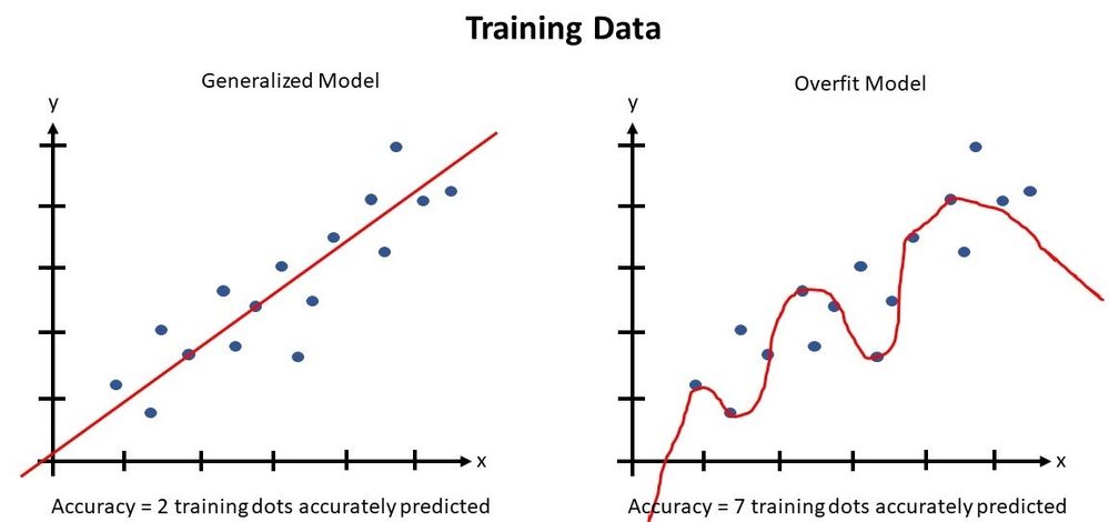
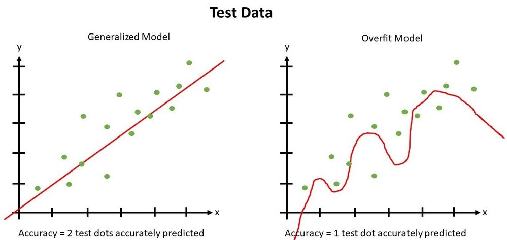
To understand what overfitting is, look at the two sets of graphs below. The blue dots represent the training data points, and the red lines represent the model function inferred from the training data that will be used to predict on new data. The top two graphs show two possible models based on the same training data, while the bottom graphs show how the same models perform on test data. On each set the left model is what we refer to as a “Generalized” Model. The red line (aka ‘model’) serves as a trend line and predicts the trend by trying to be placed in the middle of the training points on the scatterplot. It is a simple straight line defined by a first order linear equation. In the Generalized Model, the model only accurately predicts 2 of the 16 training points (shown by going through the 2 points). However, its placement minimizes the error (distance between the other points and the line). In contrast, in the Overfit Model on the right, the model employed is more complicated and defined by higher order equations. In the case of the Overfit Model, the model BETTER PREDICTS the training data, accurately predicting 7 of the 16 training data points. We might be tempted to think that the Overfit Model is better because it achieves higher Accuracy when predicting the training data; however, when the models try to predict on the previously unseen Test Data, the Accuracy of the Overfit Model underperforms that of the Generalized Model and it does not reflect the true trend of the data.
Gradient boosting is flexible in the types of target variables (dependent variables) that it can handle. It can deal with continuous numeric variables such as temperature, as well as binary variables such as 0 and 1. It can also work with categorical variables such as Yes and No, or multinomial categorical variables such as “Dog”, “Cat”, and “Mouse”.
The Gradient Boosting Machine (like the other boosting algorithms) is said to be good for imbalanced training datasets. So, for example, if a training dataset has 50% of the records with a target variable of “Y” and the other 50% has a target variable of “N”, then it is considered a perfectly balanced dataset. Balanced datasets are excellent for training, but there are many cases in which the training dataset by its very nature is highly imbalanced. For example, if we are trying to detect credit card fraud, we would have a historical dataset in which each credit card transaction is a record. The number of fraudulent transactions within those records would be a very small percentage of the total. In this case, the dataset available for training a model is highly imbalanced, which presents a difficulty for many algorithms such as Logistic Regression. It is less of a problem for the GBM, however, because of the way the algorithm focuses on error records in each tree generation, as described above.
Credit Card Fraud Data
In order to help illustrate how to use the Alteryx Boosted Model, we will use a credit card fraud detection dataset for model training. Kaggle has a sizeable dataset available, which you can download here.
This particular dataset has nearly 285,000 rows, each representing a single credit card transaction. In order to hide the personal data associated with each credit card transaction, the variables are all obfuscated by their names and normalized. It is very likely these variables are the output of a PCA (Principal Components Analysis) preprocess. PCA processes are often employed to reduce many variables down to only a few independent and regularized (normalized) variables. One of the benefits of PCA is that the smaller set of variables that are output are often obfuscated and difficult to correlate back to a known input variable (without the output reports of the PCA process). Another benefit of PCA preprocessing is that the output variables have very low collinearity, which makes them better suited for modeling.
The Kaggle credit card fraud dataset has 30 columns. The main variables are named “V1” through “V28”. Following this is the “Amount” column, which is the purchase amount, and then finally the Target Variable labeled “ClassYN”. If Class=Y, then the record represents a fraudulent transaction; if Class=N, then the record is a normal transaction. Of the 284,807 total records, only 492 (0.17%) are fraud records. This means that 99.83% of the records are not fraud hence this is a very imbalanced dataset.
In preparation for modeling, we separated the 285K records into three different datasets: one for training, one for testing, and one for final evaluation. This separation into Training, Testing, and Evaluation sets can be done through random assignment, but – especially with imbalanced datasets – it is better to split the data in a semi-random way. This ensures each sub-dataset has a representative sampling of the important types of records from the original dataset[1]. Once the full dataset is split evenly into three datasets, a T-Test (Test of Means) is performed on the target variable and the most important of the other variables (“V1” – “V28”) to ensure that each dataset is statistically similar to the original.
The Alteryx Workflow
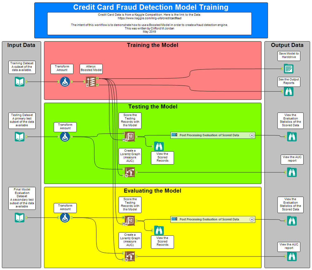
Below is a screenshot of the credit card fraud detection model and workflow created for this blog. You can download a copy of it at the Alteryx Public Gallery here.
The workflow is broken into three columns. The Input Data column on the far left, the colored processing sections in the middle, and the Output Data column on the far right. The data flows from left to right, Inputs to Outputs. The processing happens in three sections: The pink section is where the Boosted Model gets trained. In the green section, the model is tested using Test Dataset 1. The yellow section is where the final model evaluation is performed using Test Dataset 2.
Before the Training Data is used in step one of processing, we decided to transform the Amount field. Transforming variables can help the modeling process. Because the Amount field spanned from $0 to $25,000 and this scale is significantly different than the span of the variables V1 through V28, it would be best to either normalize the field or transform it to make it better correlate with the Target Variable. In this case, we decided to do a Logarithmic transformation. Specifically, the new variable “3LogAmount” is 3*Log(Amount). This transformation brings the scale to the same degree as the other variables; and, the new variable better correlates with the Target Variable (using Pearson Correlation). Because we transformed Amount for Training, we also must transform it for Testing and Evaluation.
Configuring the Alteryx Boosted Model
Required Parameters Menu
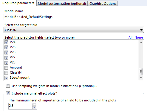
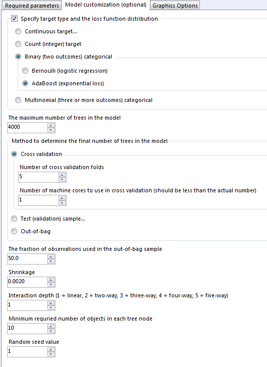
In order to configure the Alteryx Boosted Model tool, click on it in the workflow. This is what you will see in the Configuration Pane:
On the “Required parameters” tab, you can choose a Model Name. You can choose any name you want, but a good practice is to include information about how the model was configured.
Next, choose the target field. This is the field we are trying to predict. In our dataset the target field is “ClassYN”.
The next section shows a list of checkboxes for indicating the predictor fields. We check every field except Amount and ClassYN. Since we transformed the Amount field into 3LogAmount, we should check 3LogAmount, but not Amount. Also, it is very important that we do not check the ClassYN field, because it is the dependent variable and not an independent variable.
The next option is to choose whether you want to use sampling weights. If you want to do this, include a field in the data with the numeric weight for each record. For example, if there is a set of records you want to be 10 times more likely to be used than the rest of the records, then those records get weighted as 10 and the rest of the records get weighted as 1. When configuring the tool, choose the field in the dataset that has the weights. In our case, we do not need to use weights.
The next option is whether or not to include marginal effect plots. These are plots that isolate a single variable to inspect which values of that variable are most predictive of the Target Variable. These are helpful in determining how well a variable will serve as a predictor.
Model Customization Menu
Next, to further customize the model, choose the Model customization tab.
If you click on the checkbox: “Specify target type and the loss function distribution”, you can choose what type of variable the Target Value is, and then its loss function. A loss function essentially tells the algorithm how to penalize errored predictions.
Continuous target:
For example, if the target variable is continuous, there are three different loss functions available to use. A Gaussian (Squared Error Loss) function is very good to use when the predicted errors are large in value. With this loss function, since the error amount is squared, this penalizes the errors much more when they are large. A Laplace (Absolute Value Loss) function penalizes the errors linearly to their error amount. This is a faster loss function, but it does not work as well as Gaussian in cases in which the errored amounts are large.
The t-distribution loss function (AKA Student’s T loss function) should penalize errors even less than the Laplace loss function. If you choose the t-distribution, you will need to enter the number of predictive variables in the “Degrees of Freedom” field.
Count (integer) Target:
If your target variable is a count of some kind (e.g. count of sneezes a person has during allergy season), then the Boosted Model tool will automatically choose the Poisson loss function.
Binary (two outcomes) Categorical:
If you choose a target variable that is Binary Categorical, then you will have a choice of two loss functions: Bernoulli (logistic regression) or AdaBoost (exponential loss). Bernoulli has a loss function that is less steep than AdaBoost for large errors and thus penalizes such errors less. For small errors, however, Bernoulli penalizes more than AdaBoost. If your errors are large, use AdaBoost; if your errors are small, use Bernoulli.
Multinomial (three or more outcomes) categorical:
If you choose Multinomial categorical (three or more target values), then it will use a loss function geared specifically for a target variable with three or more values.
Since, in our credit card fraud use case, we have a binary categorical target (“ClassYN”), we experimented between the Bernoulli Loss Function and the AdaBoost Loss Function, because we did not know whether the errors would be large or small.
The maximum number of trees in the model:
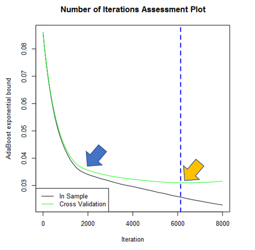
The next customization parameter that we have is the maximum number of trees. With this parameter, we want to use the minimum number of trees that will give us the best balance between processing time and error amount when tested via the Testing and Evaluation datasets. Typically, there is a value for the number of trees after which the quality of the model (measured by AUC, or Precision/Recall, or Accuracy) plateaus. In the example graph below, which was generated on the R anchor of the Boosted Model Tool, the X axis (titled “Iteration”) is the number of trees created. The Y axis titled “AdaBoost exponential bound” refers to the amount of prediction error with the number of trees. In this example, we were using an AdaBoost loss function with cross validation. There are two key points identified by the arrows in the graph.
The blue arrow identifies the “knee” of the graph. This is an inflection point where the error no longer significantly reduces as the number of trees increases. In this example, it is at about 2000 trees.
The yellow arrow identifies the “gone too far” point where the error actually begins to increase as the number of trees increases. In this example, it is at about 6000 trees.
The maximum number of trees should be between these two points on the graph. The closer to the yellow arrow point, the longer it takes to create the model, but the error will be the minimum. The closer to the blue arrow point, the less time it will take to create the model, but the error will be slightly higher. We chose right in the middle at 4000 trees.
Understand that the only way to view this graph is to run the model. So, in order to choose the optimal value for maximum number of trees, you may have to experiment by running the model with different loss functions and different values for the other parameters.
Method to determine the final number of trees in the model:
The next parameter we need to set with respect to the number of trees is the Method to Determine the Final Number of Trees in the Model. The three options are cross validation, test (validation sample), and out-of-bag. For the credit card fraud detection use case, we experimented with each method.
Cross validation:
Of the three options, the one that is consistently the best is cross validation. A recommendation for the number of cross validation folds is somewhere between 5 and 10. If the data is very noisy, you may want to increase the number of CV folds even more, to 20. Cross validation has the benefit of preventing overfitting. Unfortunately, it also takes a lot of processing power to use cross validation. This is why you can choose the number of CPU cores to dedicate to cross validation. Using more cores than the number of folds does not help, but keeping it to one core will take the longest time to process. For instance, if you have 5 CV folds, and 8 CPU cores on your machine, then you can probably up the number of cores to 4 and not significantly slow down any processing happening concurrently outside of Alteryx.
Test (validation) sample:
Using Test (validation) sample will simply tell the tool to separate out a percent of the training records (that you set) to be used for internal testing. This method is much faster than cross validation, but it is not better than cross validation.
Out-of-bag:
This method is based on the algorithm’s “out-of-bag” estimator, which typically does not reach the optimal number of trees. It is faster than cross validation and test sample, but it usually does not yield the most accurate model.
The fraction of observations used in the out-of-bag sample:
The next customization parameter is “The fraction of observations used in the out-of-bag sample” (AKA “bag fraction”). This is the percentage of training records pulled and used in each iteration of tree creation. This pulling of the records out of the bag of training records is normally random, except in the case where the random seed value is set to zero. If the random seed value is set to zero, and the bag fraction is less than one, then every time the model is retrained with the same data and the same parameters, the resulting model will be slightly different. If the random seed value is zero then it can cause that a slightly different model is built each time the workflow is run and even with the same input data. If we set it to any number (e.g. 1), and keep it on that number, then every time the workflow is run with the same input data, the model that is built will always be the same.
For the credit card fraud detection use case, we experimented with different fractions of observations to determine the optimal value.
Shrinkage:
The shrinkage value is also called the learning rate. As a general rule, the smaller the learning rate, the more accurate the model will be. But please note there are exceptions to this general rule which sometimes are encountered. Also, as a general rule, the smaller the learning rate, the longer it takes to process in an effort to reach an optimal model.
For the credit card fraud detection use case, we experimented with different shrinkage values to find the optimal value.
Interaction depth:
The interaction depth relates to how big each tree should be. There is a lot of debate on how many tree nodes and tree leaves will be formed for each value of interaction depth. What is not debated is that the greater the number, the larger each tree will be. The default value is 1 and the value that will prevent overfitting the most is a value of 1.
For the credit card fraud detection use case, we experimented with values 1 through 5 on the interaction depth to determine the best value.
Minimum required number of objects in each tree node:
The next parameter is the minimum required number of objects in each tree node. This value is the minimum number of training records that must be in each terminal node of the tree for the model to use that tree. When creating a tree, it is necessary to split the tree into right and left nodes. But before making the split official, the dataset must provide the model this minimum number of records to put in each new node. If the value is higher, this will reduce the number of tree splits that can happen and possibly reduce the number of trees. The higher the number, the more it will generalize the model and prevent overfitting. The default value is 10. The best way to know the optimal value is to experiment.
For the credit card fraud detection use case, we experimented with values 1 through 100 (the maximum possible value).
Random seed value:
Finally, the last customization parameter is the random seed value. If it is set to 0, the output models for each training run will be slightly different (even with the exact same input data). If you instead set the seed to any number greater than zero, all runs with that same seed value (and the same input data, and the same customization parameters) will yield the same output model. This is important for repeatability and testing.
Credit Card Fraud Detection Use Case
With the credit card fraud data, we ran several experiments to determine the best set of customization hyper-parameters. The first set of experiments examined the type of loss function together with the method to determine the final number of trees. The two choices for loss functions are Bernoulli and AdaBoost, and the three choices for methods are cross validation (5 folds), Test Sample (50%), and Out-Of-Bag. Below are the results.
Model Measurements
Confusion Matrix:
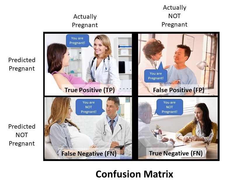
The first column is the model description. The next four columns are the “confusion matrix” values:
- TP (True Positive) means we predicted the record as fraud and it truly was fraud.
- FP (False Positive) means we predicted the record as fraud, but it was not actually fraud.
- FN (False Negative) means we predicted the record as not fraud but in reality, it was fraud.
- TN (True Negative) means we predicted the record as not fraud and it truly was not fraud.
Our main focus with the confusion matrix numbers lies with the False Positive and False Negative values: We want these to be as low as possible because they have actual costs to the company.
Please note that the confusion matrix is not an output of the Boosted Model Tool. In order to create it, we created a tool container titled “Post Processing Evaluation of Scored Data” in which we put the logic to create the confusion matrix along with the Optimal Cutoff, TotalLoss, Precision, Recall, and Accuracy fields. To find the tool container, look in the green and yellow processing sections on the right side. If you open the tool container, you can easily follow the logic.
Here is a good example to help you understand the four confusion matrix metrics:
Optimal Cutoff and TotalLoss:
After the model is created, it is fed directly into a score tool along with the Test records. The output of the score tool is a Score_Y field containing a probability that the record is fraudulent. In a default setting, if the probability is 0.50 and above, we would classify the transaction as fraud. However, by taking into account the actual costs for False Positives and False Negatives, we can calculate an optimal cutoff value that minimizes costs.
For example, if we inaccurately predict a transaction as fraudulent, the company could take an action that makes a customer upset, such as blocking the transaction and maybe even putting a freeze on the card. This could cause the customer undo stress and some will take their business elsewhere. This is the potential loss due to a False Positive.
If a card has true fraudulent transactions and yet we predict that the transactions are not fraud, then we will likely lose more money. This loss results from a False Negative. In our use case, we assigned the loss for a False Positive as $100 and the loss for a False Negative as $400. Using these values, we calculate the Optimal Cutoff score and the TotalLoss in dollars. We want the Optimal Cutoff score to be as high as possible, and the TotalLoss to be as small as possible to make sure our model is robust.
The logic for this calculation is in the tool container. There is a Text Input tool where you can set the costs for each of the categories of classifications (TP, FP, FN, and TN).
Precision, Recall and Accuracy:
These are common measurements that can be applied to models based on the results of the test data. For all of these measurements, the higher the number the better. A perfect score for each would be 1.00, although in practice that is almost never achieved.
Precision is defined as the proportion of correct positive classifications (predictions) from the cases that are predicted as positive. When False Positives rise, then the Precision declines. If our focus were to maximize detecting fraud with a concern about False Positives and with little concern about False Negatives, then Precision is a good measurement to use.
Recall is defined as the proportion of correct positive classifications from all the cases that are actually positive, which is the TP plus FN. When False Negatives rise, the Recall value declines. If our focus is on maximizing detection of all fraud with False Positives as a second priority, then Recall is the measurement to use.
Accuracy is the proportion of correct classifications (true positives and true negatives) from the overall number of cases. When we want to simultaneously measure how well our model correctly classifies “fraud” and “not fraud” transactions, then Accuracy is a good measurement to use. However, when we have a highly imbalanced training dataset
- Mark as Read
- Mark as New
- Bookmark
- Permalink
- Notify Moderator
Great article, however to run the model, I had to reduce the data set to 10% of it's original size. I presume this is due to the spec of my computer. What kind of spec would I need to be able to run this properly?
- Mark as Read
- Mark as New
- Bookmark
- Permalink
- Notify Moderator
Hello!
I have tried this on 2018.4 and 2019.02 version of alteryx, but I get the following errors:
Boosted Model (8) Boosted Model: Error in parse(text = command.string) : :1:243: unexpected symbol
I have tested to deselect all but 2 predictor fields, and I still get the error. Am I missing a package or something else required for this to run?
Kind regards
Jens
- Mark as Read
- Mark as New
- Bookmark
- Permalink
- Notify Moderator
Thank you Jensroy for pointing out the parse error. I believe the problem is with Alteryx's R Code (in the R-Tool, in the Boosted Model Macro). The code dynamically builds the R command for running the GBM (Gradient Boosted Model) algorithm. When using the T-distribution distribution loss function, the code is sticking in an extra pair of quotation marks which is causing the parse error. The 243 value marks the location of one of the bad quotation marks. Until this gets fixed, a workaround is to simply change the distribution function to either "Laplace" or "Gaussian" which are good for continuous target variables. I tested this workaround last night and it works.
Please let me know if this workaround does not work for you.
Thank you,
-cliff
- Mark as Read
- Mark as New
- Bookmark
- Permalink
- Notify Moderator
Thanks for the swift reply and an amazingly good blog post.
I will go with the new settings that you suggested.
Thanks again for the effort you put into this!
- Mark as Read
- Mark as New
- Bookmark
- Permalink
- Notify Moderator
This is great - thanks.
I'm trying to take the model results from my workflow at convert them into investment returns. As such I need the individual forecasts for each observation that goes into giving the performance metrics that I can see in the Model Comparison tool. How can I extract this data for each of the classification models (connecting a Browse Tool to the Output shows that there are usually several million bytes of data)?
Thank you in advance
- Mark as Read
- Mark as New
- Bookmark
- Permalink
- Notify Moderator
I'm running boosted model with 1.34MM records and getting the following:
Error: Boosted Model (40): Boosted Model: Error in checkForRemoteErrors(val) :
Error: Boosted Model (40): Boosted Model: Execution halted
Error: Boosted Model (40): Boosted Model: The R.exe exit code (1) indicated an error.
specified binary and adaboost
max trees 4000
5 folds, tried 4 core and 8 core
everything else at default.
If i put in a sampling tool first and select every 1 on N records (N=5000), the model runs. I have i-9 64G RAM. Is this a data or memory issue?
- Mark as Read
- Mark as New
- Bookmark
- Permalink
- Notify Moderator
RE: ebarr
With an i-9 and 64GB of RAM, I doubt seriously that it is a RAM issue even though R exit code (1) sometimes (from what I have heard) references a memory problem. What I would start investigating is if there is a specific record or records that might be causing this. I am guessing this because you say when you sample it, it works. You might smaller subsamples (eg. first 100K records) and see if it errors. If not, then the first 200K records, and so on, until you can see if it is specifically tied to specific records.
Good luck!
-cliff
- Mark as Read
- Mark as New
- Bookmark
- Permalink
- Notify Moderator
Hello! Can you kindly please provide the workflow for this mastery? 🙂 I just need a sample to try this thanks 🙂
- Mark as Read
- Mark as New
- Bookmark
- Permalink
- Notify Moderator
Great article, thank you so much for sharing! I like all the details you included here, very useful!
- Mark as Read
- Mark as New
- Bookmark
- Permalink
- Notify Moderator
Thank you for the great article
I am unable to find the workflow to learn from your work on public gallery.
Any chance you can attach along with the post here itself so it is easier to obtain the workflow?
thank you
-
2018.3
1 -
API
2 -
Apps
7 -
AWS
1 -
Configuration
3 -
Connector
3 -
Data Investigation
10 -
Database Connection
2 -
Date Time
4 -
Designer
1 -
Desktop Automation
1 -
Developer
8 -
Documentation
3 -
Dynamic Processing
10 -
Error
4 -
Expression
6 -
FTP
1 -
Fuzzy Match
1 -
In-DB
1 -
Input
6 -
Interface
7 -
Join
7 -
Licensing
2 -
Macros
7 -
Output
2 -
Parse
3 -
Predictive
16 -
Preparation
16 -
Prescriptive
1 -
Python
1 -
R
2 -
Regex
1 -
Reporting
12 -
Run Command
1 -
Spatial
6 -
Tips + Tricks
2 -
Tool Mastery
99 -
Transformation
6 -
Visualytics
1
- « Previous
- Next »
