Least Squares in an Alteryx Macro

[jdunkerley79]

A friend on the Alteryx community recently asked me about recreating the Excel trendline capabilities within Alteryx.

If you have the predictive tools installed then Alteryx has a Linear Regression tool which will fit a linear model to the set. This uses R and produces a model for the entire dataset. For my implementation, I wanted to allow for groups of data and go back to first principles and use the core Alteryx tools (i.e. no SDKs, R, or Python) to build it.

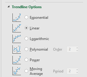
Excel has 6 options for fitting a trendline to a dataset. Apart from Moving Average these are all fitted using the least squares method. The five models are:

• Exponential:
• Linear:
• Logarithmic:
• Power:
• Polynomial:  depends on Order

For my Alteryx macro, I plan to support Exponential, Linear, Logarithmic, and Power (Moving Average isn't really the same and Polynomial will need more work).

The Excel tool also allows you to specify an intercept (the value when ) for Linear, Exponential, and Polynomial. In other words, fixing the value of A in each case. In the Power case, the intercept is always 0 and for the Logarithmic case it will be an error as the logarithm is not defined at 0. I want my macro to also support this.

Finally, you can get the trendline in Excel to output both the equation and the value of , so the last requirement is to do this as well.

A quick shout out to the LaTeX Previewer by Troy Henderson - I used it to create the SVG of all the LaTeX in this post. Onto the maths...

Least Squares Method for Regression

Let's imagine we have a dataset of points .

The goal of the least squares method is to fit a function , which minimises the square of the errors, , where   is defined as . In other words:

So, let's work this out for the Linear case. Let's expand out the summation and then see if we can simplify it:

First, substitute for :

Next, replace :

Now, expand out the square:

The goal is to find A and B to minimise the above expression:

Going back to calculus basics, a maximum or minimum will be when the first derivative is 0. So let's differentiate with respect to A:

We want to find when this is 0. Rearranging (and dividing by 2):

We can then expand the sums for this:

Dividing by n, this gives us:

Where   and  are the average of x and y respectively.

Now back to the original expression, this time let's differentiate with respect to B:

Following a similar approach, we can get that:

If we have a known intercept, then we can substitute this for A above. Otherwise, we can substitute our expression we had above for A:

This means to find A and B, all we need to compute is:

• n - the number of records
• - the average of x
• - the average of y
• - the sum of x squared
• - the sum of x times y

All of this is straight forward using the Summarize tool.

 

Building the First Macro

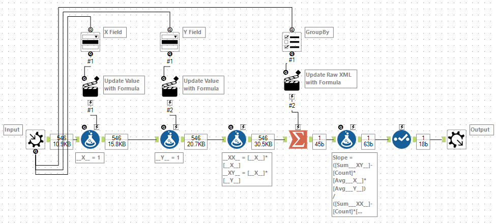
Let's start building the macro. This first version will handle computing A and B for the linear model.

We start by taking a standard macro input. I have chosen not to expose a FieldMap but instead created new variables called __X__ and __Y__. I used a dropdown box to allow you to map the field to each, using an action tool to update the raw XML of a pair of formula tools.

Next, I computed values for __XX__ and __XY__ which I needed to compute the totals. Then it was on to the Summarize tool to compute the five values I needed. Additionally, I used a List Box to allow selection of the Group By within this macro. This was a little fiddly inside the formula for action tool, but basically, it worked by adding the group by entries to the raw XML of the summarise:

IIF([#1]='""',
    '',
    '<SummarizeField field=' + 
      Replace([#1], '|||', ' action="GroupBy" /><SummarizeField field=') +
    ' action="GroupBy" />')
+
[Destination]

Finally, the last step was to compute the Slope and Intercept and to use a select tool to drop all the intermediary fields. One last little catch is to remember to select the Output fields change based on macro's configuration or data input option within the Interface Designer.

Expanding to Other Models

Currently, it can only solve Linear. However, we've basically finished the hard work and all we need to do is see how we can transform the inputs to get each of the other models.

Logarithmic:

This is straight forward. If we take the log of x as __x__ then we have the linear model.

Exponential:

Let's take the log of both sides:

Again, we have gotten to a linear model. If we take the log of y as __y__ and then take the exponential of the intercept we can compute this model.

Power:

Let's take the log of both sides:

As before, this is a linear model. In this case, we have to take both the log of x as __x__ and the log of y as __y__ and then finally take the exponential of the intercept to compute this model.

Expanded Macro

First, let's add a model drop down with a manual set of values:

Linear (y=A+Bx):Linear
Logarithmic (y=A+B ln(x)):Logarithmic
Exponential (y=Ae^(Bx)):Exponential
Power (Y=Ax^B):Power

We can feed this into a new formula tool after the one creating __X__ and __Y__ values to create the adjusted series we need.

__X__ = IIF([#1] IN ('Logarithmic', 'Power'),LOG([__X__]),[__X__])
__Y__ = IIF([#1] IN ('Exponential', 'Power'),LOG([__Y__]),[__Y__])

And then add an additional step to formula tool, adjusting the intercept for Exponential and Power:

Intercept = IIF([#1] IN ('Exponential', 'Power'), EXP([Intercept]),[Intercept])

Equation

Now that we have different models it seems a good time to add a new column containing the expression. A simple formula tool will handle this:

ToString([Intercept]) + 
IF [#1] = 'Logarithmic' THEN
 ' + ' + ToString([Slope]) + ' LOG(X)'
ELSEIF [#1] = 'Exponential' THEN
' EXP(' + ToString([Slope]) + ' X)'
ELSEIF [#1] = 'Power' THEN
' X ^ ' + ToString([Slope])
ELSE
	' + ' + ToString([Slope]) + ' X'
ENDIF

R Squared

R Squared is a measure which measures how much of the dependent variable is predicted by the model. It is expressed as:

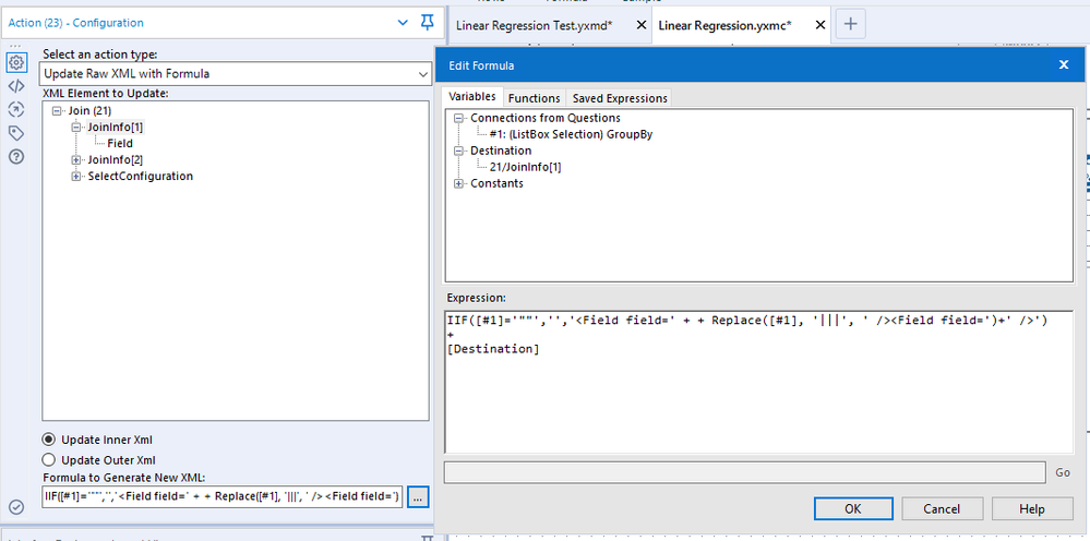
In order to compute this, I needed to join the model values back to the original series. As we might not always have a grouping field, I needed to add a dummy variable, __D__, which can be included in all joins as a common field. Dynamically creating joins is a little harder than adding group by clauses (as we must do it twice!). In this case, we need to take something that looks like "A"|||"B"|||"C" to something like:

<Field field="A" />
<Field field="B" />
<Field field="C" />

This is like the last case but needs to be applied to two nodes in the Join configuration. The expression below changes the list to the raw XML needed:

IIF([#1]='""','','<Field field=' + + Replace([#1], '|||', ' /><Field field=')+' />')
+
[Destination]

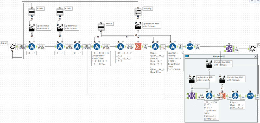
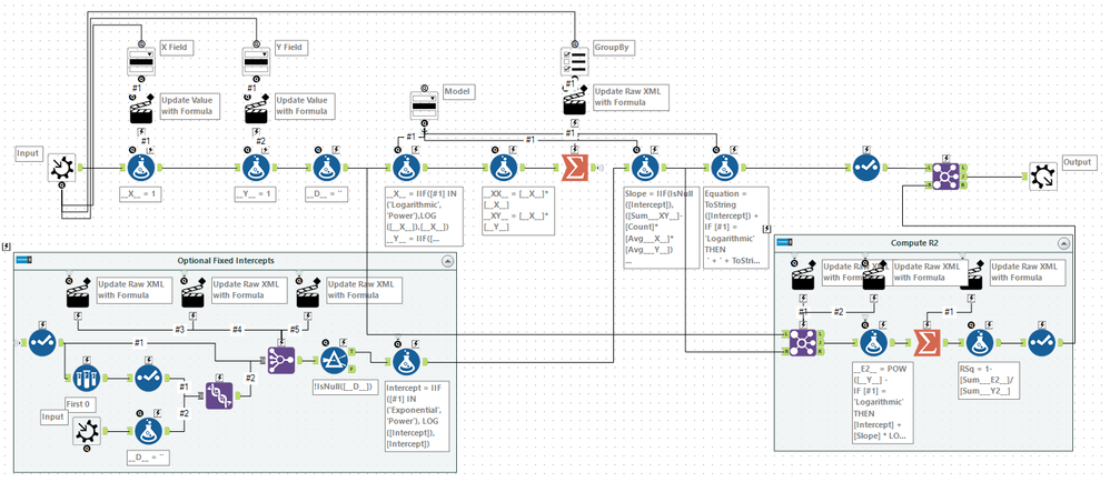
Now to compute the values we need for R squared, I first used a formula tool to evaluate the top and bottom of the fraction and then used a summarise to make totals. Again, this summarise tool needs to be grouped in the correct manner. Finally, I computed the R squared value for each set. After this, I knew that the output of this calculation would be in the same order as the output of the Slope/Intercept calculation so I joined by record position to add the value to the output. At this point the macro looked like:

Fixed Intercepts

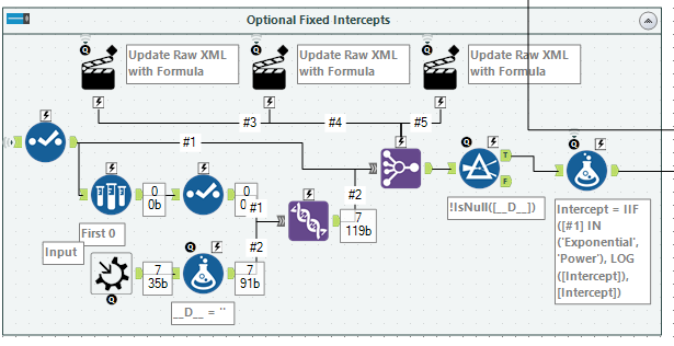
The last step was to take in an optional set of intercepts. Alteryx supports optional Macro Inputs, they will come through as an empty (0 row) copy of the template if no input is supplied. Unfortunately, as we were building the grouping fields dynamically, we couldn't have a template that would work for all cases.

The workaround I chose, was to take the output of the Summarise tool, sample 0 rows from it, and use it to create a complete set of all the columns we need. This can then be unioned to the Macro Input tool to create a superset of columns. Using similar expressions to the above, we can reconfigure a Join Multiple tool. I chose to use this over a Join tool as it meant that the order of the records from the Summarise tool was preserved.

The formula tool at the end copes with the Exponential and Power models, where the Intercept needs to be adjusted. Finally, the Slope calculation needs to be updated to use the Intercept if provided:

IIF(IsNull([Intercept]),
([Sum___XY__]-[Count]*[Avg___X__]*[Avg___Y__]) / ([Sum___XX__]-[Count]*[Avg___X__]*[Avg___X__]),
([Sum___XY__]-[Count]*[Intercept]*[Avg___X__]) / [Sum___XX__]
)

Wrapping Up

You can download the final macro here.

This macro should re-create most of the capabilities of Excel trendlines. The direct manipulation of raw XML does mean that some field names (e.g. containing a ", ||| or >) may cause it some issues.

If you want to fit another expression you can hopefully use the techniques above to get you started. Some of the techniques in building the macro are quite advanced but provide a powerful way to add new functionality.

[JamesFo]

Hi @jdunkerley79 , 

Thanks for this really interesting macro - sounds perfect for something that I wanted. Using a simple (made-up) data set, I'm getting some interesting differences between the macro and Excel, and I'm wondering if they can be easily explained. (I do appreciate that this post is from almost a year ago!!).

Using the same data set in Excel & Alteryx through your macro for two groups I get the following:

Product	Excel - Equation	Excel R²	Macro Slope	Macro R²
Product X	y = -0.001x + 10.383	R² = 0.9637	-0.000995	0.963705
Product Y	y = -3E-05x + 8.4273	R² = 0.0002	0.000482	0.051478

It is strange to me that the R2 are so different for the (poorly correlated) Product Y group (but identical for the 1st!).

I can't seem to attach files to this post, but data is as follows:

Spoiler

Using X = Units
And Y = ASP

Product	Customer	#	Customer name	Units	Revenue	ASP
Product X	Customer	1	Customer 1	1844	15674	8.5
Product X	Customer	2	Customer 2	424	4240	10
Product X	Customer	3	Customer 3	410	4100	10
Product X	Customer	4	Customer 4	203	2030	10
Product X	Customer	5	Customer 5	1059	10060.5	9.5
Product X	Customer	6	Customer 6	1836	15606	8.5
Product X	Customer	7	Customer 7	522	5115.6	9.8
Product X	Customer	8	Customer 8	1934	16439	8.5
Product X	Customer	9	Customer 9	1548	13467.6	8.7
Product X	Customer	10	Customer 10	1508	13119.6	8.7
Product X	Customer	11	Customer 11	512	5017.6	9.8
Product X	Customer	12	Customer 12	918	8904.6	9.7
Product X	Customer	13	Customer 13	1806	15351	8.5
Product X	Customer	14	Customer 14	266	2660	10
Product X	Customer	15	Customer 15	1424	12816	9
Product X	Customer	16	Customer 16	1925	16362.5	8.5
Product X	Customer	17	Customer 17	1498	13482	9
Product X	Customer	18	Customer 18	660	6468	9.8
Product X	Customer	19	Customer 19	402	4020	10
Product X	Customer	20	Customer 20	552	5409.6	9.8
Product X	Customer	21	Customer 21	182	1820	10
Product X	Customer	22	Customer 22	270	2700	10
Product X	Customer	23	Customer 23	1969	16736.5	8.5
Product X	Customer	24	Customer 24	610	5978	9.8
Product X	Customer	25	Customer 25	1274	11466	9
Product X	Customer	26	Customer 26	1574	13693.8	8.7
Product X	Customer	27	Customer 27	913	8856.1	9.7
Product X	Customer	28	Customer 28	534	5233.2	9.8
Product X	Customer	29	Customer 29	1699	14781.3	8.7
Product X	Customer	30	Customer 30	806	7818.2	9.7
Product X	Customer	31	Customer 31	869	8429.3	9.7
Product X	Customer	32	Customer 32	1751	14883.5	8.5
Product X	Customer	33	Customer 33	338	3380	10
Product X	Customer	34	Customer 34	983	9535.1	9.7
Product X	Customer	35	Customer 35	709	6948.2	9.8
Product X	Customer	36	Customer 36	354	3540	10
Product X	Customer	37	Customer 37	1520	13224	8.7
Product X	Customer	38	Customer 38	422	4220	10
Product X	Customer	39	Customer 39	1916	16286	8.5
Product X	Customer	40	Customer 40	1321	11889	9
Product X	Customer	41	Customer 41	1061	10079.5	9.5
Product X	Customer	42	Customer 42	771	7478.7	9.7
Product X	Customer	43	Customer 43	332	3320	10
Product X	Customer	44	Customer 44	801	7769.7	9.7
Product X	Customer	45	Customer 45	1707	14850.9	8.7
Product X	Customer	46	Customer 46	1742	15155.4	8.7
Product X	Customer	47	Customer 47	590	5782	9.8
Product X	Customer	48	Customer 48	319	3190	10
Product X	Customer	49	Customer 49	1826	15521	8.5
Product X	Customer	50	Customer 50	1592	13850.4	8.7
Product Y	Customer	1	Customer 1	258.8102	2070.481	8
Product Y	Customer	2	Customer 2	244.711	2447.11	10
Product Y	Customer	3	Customer 3	1860.708	14885.66	8
Product Y	Customer	4	Customer 4	1484.176	11873.41	8
Product Y	Customer	5	Customer 5	426.8291	4268.291	10
Product Y	Customer	6	Customer 6	364.6074	3281.467	9
Product Y	Customer	7	Customer 7	1673.012	13384.1	8
Product Y	Customer	8	Customer 8	48.32538	483.2538	10
Product Y	Customer	9	Customer 9	1270.204	11431.84	9
Product Y	Customer	10	Customer 10	1385.109	9695.765	7
Product Y	Customer	11	Customer 11	950.2305	6651.613	7
Product Y	Customer	12	Customer 12	62.06437	496.515	8
Product Y	Customer	13	Customer 13	127.6354	1148.719	9
Product Y	Customer	14	Customer 14	828.2687	7454.419	9
Product Y	Customer	15	Customer 15	1866.312	18663.12	10
Product Y	Customer	16	Customer 16	1595.051	12760.41	8
Product Y	Customer	17	Customer 17	96.31437	674.2006	7
Product Y	Customer	18	Customer 18	1152.339	9218.715	8
Product Y	Customer	19	Customer 19	1025.081	9225.728	9
Product Y	Customer	20	Customer 20	984.6796	8862.117	9
Product Y	Customer	21	Customer 21	645.1571	5806.414	9
Product Y	Customer	22	Customer 22	394.8476	2763.933	7
Product Y	Customer	23	Customer 23	636.0676	5088.54	8
Product Y	Customer	24	Customer 24	248.4774	1987.819	8
Product Y	Customer	25	Customer 25	1001.295	8010.364	8
Product Y	Customer	26	Customer 26	1850.038	16650.34	9
Product Y	Customer	27	Customer 27	1047.355	10473.55	10
Product Y	Customer	28	Customer 28	1152.825	9222.604	8
Product Y	Customer	29	Customer 29	149.6383	1197.106	8
Product Y	Customer	30	Customer 30	1311.027	11799.25	9
Product Y	Customer	31	Customer 31	1177.507	8242.549	7
Product Y	Customer	32	Customer 32	201.6614	1613.291	8
Product Y	Customer	33	Customer 33	982.2153	9822.153	10
Product Y	Customer	34	Customer 34	1146.483	9171.864	8
Product Y	Customer	35	Customer 35	587.773	4702.184	8
Product Y	Customer	36	Customer 36	615.1612	5536.451	9
Product Y	Customer	37	Customer 37	1935.334	19353.34	10
Product Y	Customer	38	Customer 38	369.2261	3323.035	9
Product Y	Customer	39	Customer 39	643.6709	4505.696	7
Product Y	Customer	40	Customer 40	1128.78	11287.8	10
Product Y	Customer	41	Customer 41	727.1274	6544.146	9
Product Y	Customer	42	Customer 42	302.9213	3029.213	10
Product Y	Customer	43	Customer 43	490.054	4410.486	9
Product Y	Customer	44	Customer 44	1560.278	12482.23	8
Product Y	Customer	45	Customer 45	1609.532	14485.79	9
Product Y	Customer	46	Customer 46	1122.43	10101.87	9
Product Y	Customer	47	Customer 47	627.0826	5643.744	9
Product Y	Customer	48	Customer 48	158.9554	1112.688	7
Product Y	Customer	49	Customer 49	890.6891	8016.202	9
Product Y	Customer	50	Customer 50	1911.796	19117.96	10

Best wishes,

James

[Tiers93]

Can someone please give this man a medal. This is fantastic

[Yogi]

How to created Batch Macros ?

[sjm]

This is so helpful! Exactly what I was looking for!