How To Rapidly Retrieve Data From Large Data Sets Using Alteryx

[Ken_Black]

This article originally appeared on the Data Blends blog.

Some days I feel like a billionaire! To understand why that is so, you must read this short article.

The Problem

First, let us assume you have just been given a data set with hundreds of millions or billions of records. Next, you are asked to quickly retrieve certain segments of that data. The key operative word in that last sentence is “quickly”. The final requirement is that you will have to do this type of data retrieval many times in the future.

If you are lucky, your data source is already properly partitioned to allow you to quickly retrieve the data. In many cases, however, that is not the case.

In the example I show in this article, the data is in CSV format. If you have Alteryx, there is a way for you to prepare your data for really fast data retrieval.

The Example Problem

In the following example, I’ll show how Alteryx can rapidly retrieve data. This example contains spatially-variable daily weather data from the continent of Australia. The weather data has been interpolated onto a grid, with nodes every 5 km in lat and long.

As shown in Figure 1, there are 281,963 nodes covering the continent (upper right panel). With 365 days of data per year, this equates to 102,916,495 records of data per year. With 100 years of data, this means this data source will have in excess of 10 billion records of data. In normal usage, it is expected that data from dozens to hundreds of locations will have to be extracted at any time.

Figure 1 – The Australian weather grid

The ultimate goal is to be able to rapidly pull 100 years of time series data from any location(s) on this grid. In this example, I will keep the project slightly smaller and interrogate 11 years of data, or over 1 billion records. This is a common type of application for numerical modelers that use gridded networks like finite-difference, finite-element, or other types of structure grids.

The Data Retrieval Methods

Method 1 – Alteryx (*.yxdb) files

In Alteryx, I can use two efficient methods to store and retrieve the data. In case #1, I can use a *.yxdb file to hold each year of data. As shown in Figure 2, these files are about 8.5 Gb apiece and contain 102 Million records each.

Figure 2 – The annual databases for Australia.

I could use a workflow like the one shown in Figure 3 to pull data for multiple locations. In this case, the workflow completed in 45 minutes and 8 seconds. If I only had to do this once, this time to retrieve the data might be acceptable. In cases of repetitive data retrieval, however, this amount of time would not be acceptable. Imagine if all 100 years of data were included – you would be waiting for 7.5 hours to retrieve the data!


Figure 3 – Workflow used to pull 11 years of time series data from 14 locations. This took over 45 minutes to execute.

Method 2 – Calgary (*.cydb) Files

However, if you have the need to pull data many times, the better data storage method would be to use Calgary files. Figure 4 shows how you create Calgary files in Alteryx.


Figure 4 – This shows how to use the Calgary loader tool to create a Calgary file in Alteryx. Note that the index fields I selected are the Record ID (location ID), the day of the year (1-366), the latitude and longitude. These indexes are the key to allowing rapid data retrieval, so you need to choose them wisely. Notice that you can also deselect data so that it will not be available in the Calgary file.

Once your Calgary files are created, there will be multiple files for each. As shown in Figure 5, there are a total of six files for one year (2019) of my example data. The *.cydb file holds the data and the other files contain information on the indices.

Figure 5 – One year of Calgary files for this example. The time taken to create this indexed structure was 9 minutes and 22 seconds. This is a one-time penalty for creating these file unless you plan to refresh the data. In this case of historical data, the Calgary files only need to be created once.

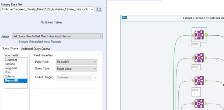
Once all 11 indexed files are created, the workflow shown in Figure 6 was used to extract 11 years of data from the 14 locations. As can be seen, this took under 6 seconds, compared to over 45 minutes with the *.yxdb example shown in Figure 3. Remember, this is retrieving over 53,000 records from over 1 billion records. For the full case of 100 years, the Calgary extraction method will run in about 1 minute, versus 7.5 hours for the *.yxdb method.

Figure 6 – The workflow used to retrieve the data from 14 locations. The detailed configuration of the Calgary join tools are shown below.

You configure the join operation as shown in Figure 7. The configuration is very simple with an alignment made between your input fields and the indexed fields. In this case, I am only using the RecordID field to retrieve the data.

Figure 7 – The Calgary join tool configurations. Note that the join is being done using only the RecordID field. You align the input field with one or more of you indexed fields. The action setting also allows you some flexibility in what you receive from the join operation.

If you want to learn some additional specific techniques for this methodology, I strongly encourage you to read this article. That article shows how a batch file can be used to automate the process of creating multiple Calgary files. It also includes another example of using Calgary files for some big data.

Visualizing the Data

Once the weather data has been retrieved, it can be visualized as shown in Figure 8.

Figure 8 – An example dashboard showing the data from one location over time

Final Thoughts

The Calgary data storage methodology is a very important tool in the Alteryx arsenal. I think it is underutilized, so I hope this article inspires people to try it for themselves.

Now the answer to my earlier statement of why I feel like a billionaire! Well, easily working with really large data sets like the one I showed in this article makes me feel happy and satisfied. Earlier in my career, it was a struggle to use billion+ line files. Trying to visualize this much information was very tough. Now thanks to Alteryx and Tableau, using billion+ record files is easy and somewhat common for me to do.

This makes me feel like a billionaire! Thanks for reading!