Data Science
Machine learning & data science for beginners and experts alike.- Community
- :
- Community
- :
- Learn
- :
- Blogs
- :
- Data Science
- :
- Alteryx Data Science Design Patterns: Predictive ...
- Subscribe to RSS Feed
- Mark as New
- Mark as Read
- Bookmark
- Subscribe
- Printer Friendly Page
- Notify Moderator
In our second post we introduced the idea of a generating process and its true functional form. Let’s continue the discussion by reviewing the sixth component of a prescriptive model: the induction algorithm.
An analytical model’s induction algorithm is the algorithm that approximates the true functional form of the modeled generating process. Once we have fitted the induction algorithm to the generating process, we can use the fitted induction algorithm to estimate the value of the dependent variable for new sets of independent variables. (In classical statistical modeling, this estimation process is sometimes termed scoring. We’ll stick with the more general terms estimation and prediction.)
Parametric Statistical Induction Algorithms
When a model is a parametric statistical model, the induction algorithm is an equation specifying the value of the dependent variable as a function of the independent variables, plus some noise. For example, a linear model of percent body fat (PBF) as a function of the predictors we saw in our previous post might have the following general form:
PBFi = β0 + β1agei + β2weight_lbsi + β3BMIi + εi
This equation gives us the PBF of person i as a linear combination of that person’s other attributes, plus a person-specific error term. If we rename the named variables (age, weight_lbs, and BMI) with deliberately meaningless names of the form xj, and if we assume (as is common) that the error terms are independent and identically distributed (iid), the above equation becomes a model formula:
PBFi ~ β0 + ∑βjxij
where you can read the tilde to mean “is distributed as.” (The R language has a slightly different concept of a model formula.)
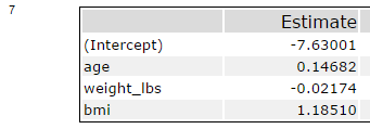
The first formula above is deterministic; if we magically knew in advance how far off the model’s prediction would be for each person (the values of the error terms), we could calculate each person’s PBF exactly. The second formula is stochastic (statistical). It acknowledges that we don’t know the error in advance. Rather, we assume (and later check) that the error terms have a certain statistical distribution. (This assumption is central to the concept of a parametric statistical model.) In the case of an ordinary least squares (OLS) linear regression, we assume the distribution is normal (the usual “bell shaped” distribution) with zero mean. That leaves us having to estimate the error terms’ variance σ2. We must also estimate the intercept term β0 and the coefficients βj. Each of these quantities requiring estimation is a parameter of the induction algorithm. So an OLS linear regression has two more parameters than it does variables. This illustrates another important property of parametric statistical models: the number of parameters varies with the number of model features. Estimating these parameters’ values is precisely what we mean by fitting a parametric model. For example, the first OLS linear model we fitted in our previous post appears in row seven of the model output. The βj values are in the column with the heading ‘Estimate’:
Figure 1: Parameter Values for OLS Model Predicting PBF
The model formula is thus (with some rounding)
PBFi ~ -7.630 + 0.147 × agei – 0.022 × weight_lbsi + 1.185 × BMIi
Statistical Induction Algorithms that are not Parametric
Many statistical induction algorithms are not parametric. Oddly, this does not mean they don’t have parameters. It means that the size of the set of parameters varies in some other way, often depending on the quantity of data. Such induction algorithms can be semi-parametric, semi-nonparametric, or non-parametric. Eventually we will delve into design patterns using these statistical distinctions. For now, let’s turn our attention to machine-learning induction algorithms.
Machine-Learning Induction Algorithms
The distinction between machine-learning and statistical models is often largely historical, aligning an analytical method with the academic discipline that created the method, rather than with a method’s formal properties. Machine-learning methods originally were products of artificial-intelligence (AI) research within the computer-science discipline. AI’s early failures to produce general artificial intelligence led researchers to focus on the more narrow task of making a computer learn how to solve a specific class of similar problems. The result was machine-learning models.
It’s important to recognize that statistical models “learn” an approximation to a generating process’ true functional form just as much as machine-learning models. (That learning is what lets us use both statistical and machine-learning induction algorithms to predict.) The key formal difference is that most statistical models learn by fitting an explicit, approximate functional form; while machine-learning models fit an induction algorithm without explicitly specifying an approximate functional form. The functional form is only implicit in the induction algorithm’s behavior.
Let’s look at an example. Decision trees are a widely used family of machine-learning models for supervised classification (predicting class membership for a known set of classes) and regression (predicting a numerical value). A classification tree is a decision tree used for supervised classification. When we fit a classification tree to a given set of problem features and input data, we specify how many nodes and branches the tree has, how they connect, what decisions occur at each internal node, and which class we predict at each leaf node.
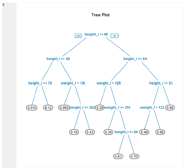
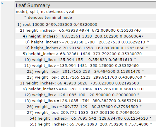
For example, Figures 2-4 below present an Alteryx classification-tree model, and model output, predicting gender on the basis of age, height, and weight (though the fitted model actually ignores age):
Figure 2: Classification-Tree Model
Figure 3: Fitted Classification Tree
Figure 4: Classification-Tree Decision Rules
The fitted tree (Figure 3) has 11 internal nodes and 12 leaf nodes. Figure 4 presents the decision rule leading to each node from its parent node. (The decision rules in Figure 3 round the numbers in Figure 4, so they fit on the diagram.) The proportions under the leaf nodes are proportions of the individuals classified by the node that are female. Assuming that misclassification of males and females has the same cost, the decision rule at a leaf node (the prediction) would be to classify an individual at that node as female if the proportion at the node was at least 0.5.
It’s interesting to consider how we might express the decision rules in Figures 3 and 4 as an explicit function, assuming we “labeled” females as ones and males as zeros. The decision at each internal node can be represented as an indicator variable that indicates whether a model feature is at least some threshold value. The thresholds are model parameters. Additional parameters could indicate whether the proportion at a given leaf node is at least 0.5. The path from the root node to a leaf node would then induce a value representing a classification. For example, the path from the root node to the leftmost leaf node in Figure 3 can be represented like this:
Ih≥66 × Ih≥68 × Ih≥70 × 0
This expression says, “If the eight is at least 66 and the height is at least 68 and the height is at least 70 then the individual is male.” We can simplify the expression for two reasons. First, the third indicator subsumes the first two, so the expression simplifies to
Ih≥70 × 0
Second, multiplying by zero yields zero, regardless of the values of the indicator variables; so the expression is always zero. In a similar fashion the path from root to the rightmost leaf node reduces to
Ih≥70 × 1
(A third type of simplification is possible when an internal node is the parent of two leaf nodes having the same class value: one can drop the leaf nodes, and convert their parent to a leaf having the class value. The first and second leaf nodes illustrate this simplification. Both nodes have the class value of zero, that is male; so we could delete those nodes and treat their parent as a male leaf node.)
The overall decision function is the sum of expressions such as the above, each expression representing a path from root to leaf. Exactly one of these expressions will have indicator values that all evaluate to one, and the leaf’s value will be a zero or a one; so at most one expression will evaluate to a one, and the others to zeros. The zero-valued leaf nodes’ expressions cannot affect the value of the sum, so we only need to include the expressions for leaf nodes that evaluate to one. As a notational convenience, we can define the inverse of an indicator variable as I-1 = (I – 1)2. So for example, Ih≥66-1 = Ih<66. The function is then
f(i) = Ih≥66-1 × Ih≥64 × Iw<126-1 × Iw≥210-1 + Ih≥63 × Iw<123-1 + Ih≥63-1
after applying the three types of simplifications outlined above, and expressing the indicator variables and their decision rules as they appear in the tree diagram (some of them using ≥ and others <).
We have thus illustrated a method for converting a classification tree into an explicit approximating function. The conversion involves converting the tree model’s features to a set of indicator variables, applying some simplifications, and then converting the paths from root to leaf nodes into products of indicator variables. There is one indicator variable per node in the tree, hence one indicator variable (feature of the transformed model) per parameter. This begs the question whether the transformed model counts as a statistical model. Most statisticians would say no, because the approximating function does not explicitly represent model uncertainty with random variables. You might think about whether and how one could do so, and whether the result would be a parametric statistical model.
Distinguishing a Model from its Induction Algorithm
Understanding or expressing many data-science design patterns depends strongly on one’s ability to distinguish a model from the induction algorithm used in the model. For example, the classification tree’s induction algorithm takes a fitted tree and then traverses it from the root node to a leaf node once for each new input record, and classifies the new input as belonging to the class predicted for the leaf node. This procedure says nothing about how we chose the classification tree’s input variables, how we transformed those variables to produce the model’s features, or how we computed the fitted tree’s structure. These “hows” are part of the model, but not part of the induction algorithm. The induction algorithm just tells us how to use the fitted model to predict. Unfortunately the data-science world often conflates the two concepts. Now you know better!
You must be a registered user to add a comment. If you've already registered, sign in. Otherwise, register and sign in.


