Data Science

TimothyL · ‎04-18-2019

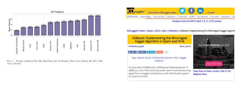
In 2017, Randal S. Olson published a paper using 13 state-of-the art algorithms on 157 datasets. It proved that gradient tree boosting models outperform other algorithms in most scenarios. The same year, KDNugget pointed out that there is a particular type of boosted tree model most widely adopted. More than half of the winning solutions in machine learning challenges in Kaggle use xgboost.

Let's Start

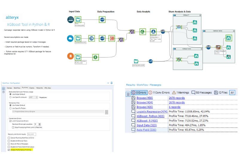
In this example, we explore how to use XGBoost through Python. Certainly, we won't forget our R buddies! Download the sample workflow with both R & Python macro.

If you never heard of it, XGBoost or eXtreme Gradient Boosting is under the boosted tree family and follows the same principles of gradient boosting machine (GBM) used in the Boosted Model in Alteryx predictive palette. The key differences include:

Regularised to prevent overfitting, giving more accurate results; and
A sparse matrix data structure, giving more efficient cache utilisation and processing speed

Thanks to this beautiful design, XGBoost parallel processing is blazingly faster when compared to other implementations of gradient boosting.

Kaggle image

To use the XGBoost macro, you need to install the libraries (xgboost, readr, etc) for both R & Python macro to work. Here are the links for R & Python guideline if you are new to this, look for the below error message then install the corresponding library.

Once the packages are installed, run the workflow and click the browse tool for the result. You can also Enable Performance Profiling (on the Runtime tab of the Workflow - Configuration window) to check how fast the XGBoost completes, compared with the traditional logistic regression.

After running it, you might want to use the tools for the other use cases immediately. But wait! Hold on, let's learn how to prep your data and interpret your output first.

Data Input

As with our other predictive tools, connect your training data to the I anchor, and your new raw data stream (which does not contain the target variable) to the D anchor.

A few things to consider:

XGBoost only supports numeric values. You need to transform the categorical features with one hot encoding, mean encoding, etc. Don't know how to do it? I got one for you!
Use the Imputation Tool to fill all the missing, blank & null values
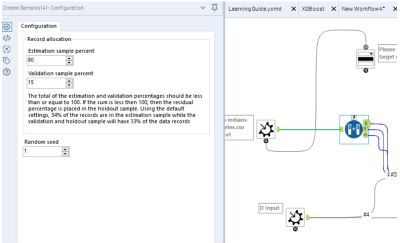
No need split into validation & holdout sets, the tools do it for you. Change the split ratio? Just open the macro and modify the Create Sample Tool.

Report & Score Output

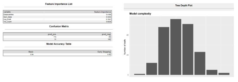
The R anchor is the model report, which presents to you key insights:

Which variable is the most crucial factor in Feature Importance Table
How accurate is the model in Accurate Metric Table
What is the model complexity in Tree Plots

S anchor is the scored result using the testing data. The reason we are not using the score tool here is XGBoost transforms data into sparse matrix format, where our score tool has to be customised. In case you want to save the model object and load it in another time, go to the additional resource at the bottom.

Hyper-Parameter Optimisation (HPO)

After setting up the variable, there are some extra parameters to fine-tune the model. In fact, there are hundreds! Such as defining your optimisation objectives, evaluation criteria, loss function, more and more. It's this level of flexibility that makes every data scientist addicted to it.

I only carve out some critical parameters in the configuration box, feel free to jump inside the macro and enrich the settings based on your need. If you are new to the Alteryx interface tools and macros, please check out our chief scientist Dr. Dan's Guide to Creating Your Own R-Based Macro Series.

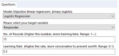
R Configuration:

R Code:

md <- xgb.train(data = dxgb_train, nthread = n_proc, 
          objective = "%Question.objective.var%", nrounds = %Question.roundno.var%, 
          max_depth = 20, eta = %Question.lr.var%, 
          min_child_weight = 1, subsample = 0.5,
          watchlist = list(valid = dxgb_valid, train = dxgb_train), 
          eval_metric = "auc",
          early_stopping_rounds = 10, print_every_n = 10)

To save your time, here is a summary table with parameter info and tuning tips. Hot sauce highlighted are the ones in configuration box.

Define the problem & evaluation:

Objective / Learning Task

Linear regression (reg:linear)
Logistic regression for binary classification (binary:logistic)
Softmax for multi-class classification (multi:softprob)

Evaluation Metrics:

AUC - Area under curve (used in classification)
RMSE - Root mean square error (used in regression)
merror - Exact matching error, (used in multi-class classification)

Parameters to control over fitting:

Learning rate or eta [default=0.3][range: (0-1)]

Makes the model more robust by shrinking the weights on each step.
Lower eta leads to slower computation, higher eta rate avoid over-fitting but less accurate result
If time allows and model performance is key, decrease incrementally the eta rate while increasing the no. of rounds
Optimal values lie between 0.01 - 0.3

Max_depth [default=6][range: (0,Inf)]

It controls the depth of the tree.
Larger the depth, more complex the model; higher chances of overfitting.
There is no standard value for max_depth. Larger data sets require deep trees to learn the rules from data.

Parameters for speed

No of rounds/tree: [default=10][range: (1, Inf)]

It controls the maximum number of iterations
For classification, it is similar to the number of trees to grow

Sub-sample[default=1][range: (0,1)]

It controls the number of samples (observations) supplied to a tree.
Typically, its values lie between (0.5-0.8)

Early Stopping:

If NULL, the early stopping function is not triggered.
If set to an integer k, training with a validation set will stop if the performance doesn’t improve for k rounds.

Hyper-Parameter Optimisation (HPO)

Don't get panic when you see the long list of parameters. These days, there are many packages out there to help data scientist to auto-tune the model. From very simple random grid search to Bayesian Optimisation to genetic algorithms. Inside the python macro, there is a snippet of random search code for you to try. For example, modify the number iteration to 400 or the Learning Rate range to 0.01,0.2.

xgb_model = xgboost.XGBClassifier()

params = {
    "colsample_bytree": uniform(0.7, 0.3),
    "gamma": uniform(0, 0.5),
    "learning_rate": uniform(0.03, 0.3), # default 0.1 
    "max_depth": randint(2, 6), # default 3
    "n_estimators": randint(10, 100), # default 100
    "subsample": uniform(0.6, 0.4)
}

search = RandomizedSearchCV(xgb_model, param_distributions=params, random_state=42, n_iter=200, cv=3, verbose=1, n_jobs=2, return_train_score=True)

search.fit(X_train, y_train)

report_best_scores(search.cv_results_, 1)

Then the best parameter set is produced:

End. And?

That's all for now. In this post, we learned some basics of XGBoost and how to integrate it into the Alteryx platform using both R and Python. Once you feel ready, explore more advanced topics such as CPU vs GPU computation, or level-wise vs leaf-wise splits in decision trees. Below gather some materials. Enjoy.

Additional resources:

DataCamp XGBoost Course
KDNuggets: A top machine learning on Kaggle
Analytic Vidhya: An End-to-End Guide to XGBoost
Math geeks can go to the algorithm paper written by Tian Qi Chen.

What's next? LightGBM!