Alteryx Designer Desktop Knowledge Base
Definitive answers from Designer Desktop experts.- Community
- :
- Community
- :
- Support
- :
- Knowledge
- :
- Designer Desktop
- :
- Alteryx for Excel Users: How to do a VLOOKUP in Al...
Alteryx for Excel Users: How to do a VLOOKUP in Alteryx
- Subscribe to RSS Feed
- Mark as New
- Mark as Read
- Bookmark
- Subscribe
- Printer Friendly Page
- Notify Moderator
11-15-2016 02:45 PM - edited 08-31-2022 12:34 AM
VLOOKUP is one of the most commonly used functions is Excel. VLOOKUP takes a lookup value and finds that value in the first column of a lookup range. Complete the function's syntax by specifying the column number to return from the range. In other words, VLOOKUP is a join. One column of data is joined to a specified range to return a set of values from that range.
The objective of this posting is twofold:
1. Demonstrate how a VLOOKUP can be done using Alteryx.
2. Demonstrate how a VLOOKUP can actually be easier to do in Alteryx.
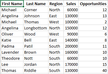
For the sake of argument, let's say we have two worksheets in one Excel file. Sheet 1 contains a master list of sales data. The data looks like this:
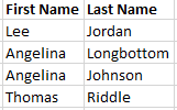
Sheet 2 contains a select list of sales people and contains First Name and Last Name:
Using a VLOOKUP function, we want to take the list of sales people, match it to sales peoplefound in Sheet 1 and return sales data for each sales person. Notice our list of sales people in Sheet 2 has two sales people named'Angelina'. Sheet 1 has multiple people named'Angelina' and 'Michael'. Using First Name alone will not return reliable results using VLOOKUP. Further, matching on Last Name - or even a concatenation of both First Name and Last Name - isn't always reliable either. There are a lot of 'Michael Thomas's in the world and several may exist in your data range. The best way to complete our VLOOKUP is to use a unique identifier for each sales person. But again, for the sake of argument, let's say each First Name and Last Name combination produces a unique name/identifier.
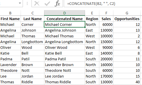
The first thing we need to do is do is concatenate First Name and Last Name in a new field.
We'll do the same thing with our data in Sheet 2. For VLOOKUPs to work properly, the data must be sorted. In our case, we'll sort both Sheet 1 and Sheet 2 in ascending order on 'Concatenated Name':
Now we're ready to use our =VLOOKUP function:
It worked! Let's see how do the same thing in Alteryx. (Hint: there's more than just one way to do it).
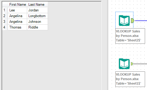
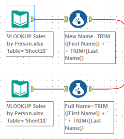
We'll start by bringing in our data from Sheets 1 and 2:
As with the Excel example, we'll concatenate First Name and Last Name in a new field. For clarity, let's name the concatenated name in Sheet 1 'Full Name' and Sheet 2 'New Name'. We'll do this using a Formula Tool expression:
Finally, let's attach a Find Replace Tool where Sheet 2 attaches to the 'F' input of Find Replace and Sheet 1 attaches to the 'R'.
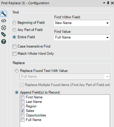
The configuration for the Find Replace looks like this:
Notice 'Sales' is selected under 'Append Field(s) to Record'. When we run the workflow, we get the sales data by sales person just like we did in Excel:
But there's an even simpler way to perform a VLOOKUP in Alteryx! Simply join the two Sheets with a Join Tool.
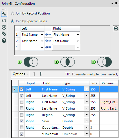
Take a look at how the Join is configured:
We joined our data on First Name andLast Name without having to concatenate the two fields first. Further, we selected the sales data we want returned in the same Join Tool.
Alteryx has an added advantage over Excel's VLOOKUP function. Let's say you want to return Sales and Opportunities. With Alteryx, this can be handled in a single Join. With Excel, we would need to do multiple VLOOKUPs.
- Mark as Read
- Mark as New
- Bookmark
- Permalink
- Notify Moderator
Also, if you put the unique tool you can essentially create a "look up table" to join with the file that you are trying to fill in.
- Mark as Read
- Mark as New
- Bookmark
- Permalink
- Notify Moderator
Hi,
I am stuck on one thing. Let's say I have two data first is (client name and amount) and second is (client name and cities). I have got city names for some clients, not all.
I want to bring city names to my first data without eliminating clients which don't have cities.
When I do it with "join" tool, it brings me intersection, or data not covered on either side. (you know "join" tool has three output options). How can I solve this problem?
Thank you
Note: I can do it by "find & replace" tool, just want to learn how to do it with "join".
- Mark as Read
- Mark as New
- Bookmark
- Permalink
- Notify Moderator
Use a union tool to append the rows from the intersection and the rows from either L or R whichever has the remaining data
- Mark as Read
- Mark as New
- Bookmark
- Permalink
- Notify Moderator
Hi
If someone can help me in putting a vlookup.
I have two sheet
Sheet 1 Info
GL Account
1001
1002
1003
1004
Sheet 2 Info
GL AccountCorresponding GL
1001
1002
1003
1004
1005
- Mark as Read
- Mark as New
- Bookmark
- Permalink
- Notify Moderator
Hi
If someone can help me in putting a vlookup.
I have two sheet
Sheet 1 Info
GL Account
1001
1002
1003
1004
Sheet 2 Info
GL Account Corresponding GL
1001 2345
1002 4234
1003 77789
1004 12345
1005 2564
Now I want to use vlookup similar to excel to get Corresponding GL from Sheet 2 to sheet 1 in different column
Thanks
Virender
- Mark as Read
- Mark as New
- Bookmark
- Permalink
- Notify Moderator
Virender,
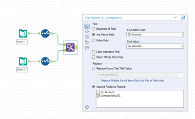
This could be done in various ways. I have used the Find & Replace tool. PFB the screenshot.
Hope this helps.
Best,
Raghav
- Mark as Read
- Mark as New
- Bookmark
- Permalink
- Notify Moderator
Awesome Knowledge.
-
2018.3
17 -
2018.4
13 -
2019.1
18 -
2019.2
7 -
2019.3
9 -
2019.4
13 -
2020.1
22 -
2020.2
30 -
2020.3
29 -
2020.4
35 -
2021.2
52 -
2021.3
25 -
2021.4
38 -
2022.1
33 -
Alteryx Designer
9 -
Alteryx Gallery
1 -
Alteryx Server
3 -
API
29 -
Apps
40 -
AWS
11 -
Computer Vision
6 -
Configuration
108 -
Connector
136 -
Connectors
1 -
Data Investigation
14 -
Database Connection
196 -
Date Time
30 -
Designer
204 -
Desktop Automation
22 -
Developer
72 -
Documentation
27 -
Dynamic Processing
31 -
Dynamics CRM
5 -
Error
267 -
Excel
52 -
Expression
40 -
FIPS Designer
1 -
FIPS Licensing
1 -
FIPS Supportability
1 -
FTP
4 -
Fuzzy Match
6 -
Gallery Data Connections
5 -
Google
20 -
In-DB
71 -
Input
185 -
Installation
55 -
Interface
25 -
Join
25 -
Licensing
22 -
Logs
4 -
Machine Learning
4 -
Macros
93 -
Oracle
38 -
Output
110 -
Parse
23 -
Power BI
16 -
Predictive
63 -
Preparation
59 -
Prescriptive
6 -
Python
68 -
R
39 -
RegEx
14 -
Reporting
53 -
Run Command
24 -
Salesforce
25 -
Setup & Installation
1 -
Sharepoint
17 -
Spatial
53 -
SQL
48 -
Tableau
25 -
Text Mining
2 -
Tips + Tricks
94 -
Transformation
15 -
Troubleshooting
3 -
Visualytics
1
- « Previous
- Next »
