Analytics
News, events, thought leadership and more.- Subscribe to RSS Feed
- Mark as New
- Mark as Read
- Bookmark
- Subscribe
- Printer Friendly Page
- Notify Moderator
In Part 1 of this series of blog posts, I compare the demographic, socioeconomic, and religious participation of the most Democratic and Republican counties in the country. This comparison was very informative, but it did not provide a good indication of the relative importance of the different factors identified. Moreover, it does not make use of all the available data. Consequently, in this post I present the results of a predictive model that was developed to predict the county level Partisan Voting Index (or PVI) following the 2012 presidential election.1
“…in this post I present the results of a predictive model that was developed to predict the county level Partisan Voting Index (or PVI) following the 2012 presidential election.”
The variables used as predictors in the model include the ones discussed in both Part 1 and Part 2 of this series, as well as ones related to age, educational attainment, and the presence of children in households. Age is included based on the notion that younger voters are more liberal and older voters are more conservative, while the educational attainment levels of a county's population age 25 and above is included since recent work suggests that those with a professional or graduate degree are becoming increasingly liberal, while those with a high school education or less tend to be more conservative.
Surprisingly, I am unable to find any work that examines the effect of the presence of children on political behavior. However, there are reasons to believe that the presence of children in a household should influence household members' voting behavior on both symbolic predisposition and economic self-interest grounds, albeit, with opposite effects. From a symbolic predisposition perspective, the transition to parenthood often results in household members taking more traditional gender roles, which would tend to result in more conservative (Republican) symbolic predispositions (the topic of Part 2 of this series). In contrast, economic self-interest would tend to result in a more liberal bias associated with federally supported childcare, family leave, and college education financial support benefits which would provide direct material well-being to households with children, and are associated with the policies of the Democratic Party.
One demographic factor that has consistently been shown to influence political preference is gender. Given the nature of gender (that the ratio starts out slightly skewed towards males, but skews increasingly more toward females with age), this variable isn't amenable to the examination of partisanship at the county level since it will be confounded with age.
The specific predictor variables used in the model are:
- The region of the country in which the county is located, where the regions are defined using Nate Silver's political region map
- The racial and ethnic makeup of each county measured as the percentage of each county's population that is non-Hispanic white, Hispanic white, African American, Native American or Alaskan Native, Native Hawaiian or Pacific Islander, Asian, non-Hispanic members of some other race, Hispanic member of some other race (a large percentage of all Hispanics fall in this group), and are of two or more races
- The age makeup of a county as measured by the percentage of the voting age population that is age 18 to 29, 30 to 39, 40 to 49, 50 to 59, 60 to 69, and 70 and above
- The presence of households with children in a county as measured by the percentage of households with members age 18 years or younger present
- The educational attainment of each county as measured by the percentage of the population 25 and over that has less than a high school education, a high school graduate or a GED holder, some college or an Associate's degree, a Bachelor's degree, and a professional or graduate degree
- The income distribution of a county as measured by the percentage of households with annual incomes under $10,000, between $10,000 and $19,999, between $20,000 and $29,999, between $30,000 and $39,999, between $40,000 and $49,999, between $50,000 and $59,999, between $60,000 and $74,999, between $75,000 and $99,999, between $100,000 and $124,999, between $125,000 and $149,999, between $150,000 and $199,999, between $200,000 and $249,999, between $250,000 and $499,999, and $500,000 and above.
- Religious participation in a county as measured by the total members of all religious congregations as a percentage of the county's population; and the share of the religious congregation members that are Evangelical or LDS, Catholic, mainline protestant (e.g., Methodist, Lutheran, Episcopal, Presbyterian), black protestant (e.g., the African Methodist Episcopal Church), Orthodox (e.g, Greek Orthodox, Russian Orthodox), or congregations that fall in the "other" category (e.g., non-Christian faiths)
“A training/test methodology is used to select between the different modeling algorithms used”
A training/test methodology is used to select between the different modeling algorithms used. The data consists of the PVI for the 3113 counties in the 2012 US Presidential election, which is divided into a training sample with 2179 records and a test sample with 934 records (a 70-30 split).2 The algorithms examined are linear regression (Alteryx's Linear Regression tool), recursive partitioning decision trees (Alteryx's Decision Tree tool), the random forest model (Alteryx's Forest Model tool), gradient based boosting (Alteryx's Boosted Model tool), and feed-forward neural networks (Alteryx's Neural Network tool). Based on the training/test methodology, the final model selected, using test sample efficacy measures, is a Boosted Model with up to four-way interactions.
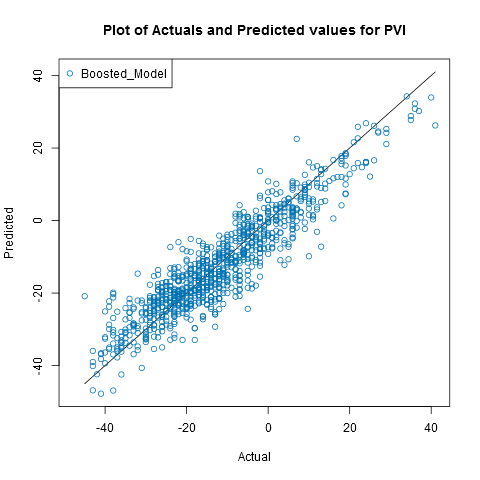
“Overall, the model displays a high degree of predictive efficacy in the test sample, with a correlation between actual and predicted values of 0.92, a root mean square error of 5.9, and a mean absolute error of 4.6”
Overall, the model displays a high degree of predictive efficacy in the test sample, with a correlation between actual and predicted values of 0.92, a root mean square error of 5.9, and a mean absolute error of 4.6. The residual plot (below) suggests the model fits well. Based on this, it appears that county level PVI values can be readily predicted using demographic, socioeconomic, and religious participation variables.
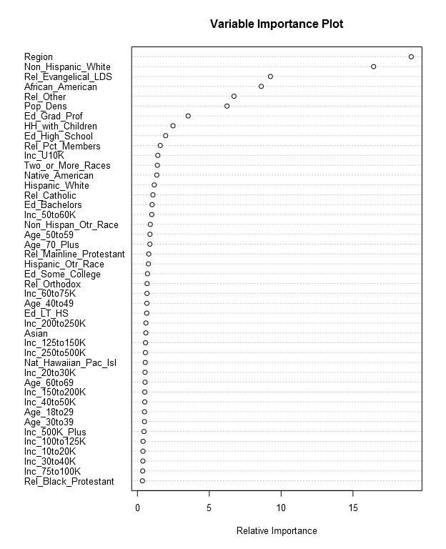
The figure below provides the variable importance plot for the selected Boosted Model. In the figure, the total importance weights sum to 100. The figure reveals that Region and the percentage of the population that is non-Hispanic white are the two most important predictor variables, each having a relative importance score of over 15. The next group, with relative importance scores around 10, is the share of religious congregation members that are either Evangelicals or LDS, as well as the percentage of the population that is African American. Following this, with relative importance scores around 8, is the percentage of religious congregation members that belong to the "other" (largely non-Christian) group, and the population density of the county (an indicator of whether a county is rural or urban in nature). Rounding out the top tend in terms of importance is the percentage of the population 25 and over with a graduate or professional degree, the percentage of households with children present, the percentage of the population 25 and over with a high school or equivalent education, and the percentage of the population that is a member of a religious congregation.
The first income variable (the percentage of households with an income below $10,000) is the 11th most important variable (with a relative importance score around 2), and the next income variable is the 17th most important variable (with a relative importance score of around 1). Perhaps surprisingly, the most important age variable is 19th on the list, with a relative importance score around 1.
“Taken together, and consistent with the comparison of the most Democratic and Republican leaning counties, the model indicates that the three most important factors in terms of driving partisanship at a county level are the three Rs….”
Taken together, and consistent with the comparison of the most Democratic and Republican leaning counties, the model indicates that the three most important factors in terms of driving partisanship at a county level are the three Rs of region, race, and religion. Looking at the sum of importance weights for different variable groups reveals that nearly 68% of the importance weight values are for the three Rs (race at 33%, region at 20%, and religion at 15%). The other factors that come into play is the educational attainment of the adult population age 25 and older and the percentage of households where children are present. While they have some effect, age and income appear to play a small role in determining the partisan nature of a county. In addition, and consistent with past empirical research, factors that are more closely associated with symbolic predispositions are substantially more important than those associated with economic self-interest.
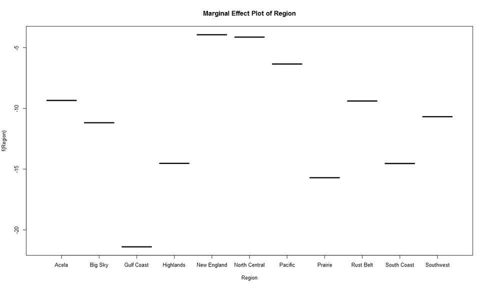
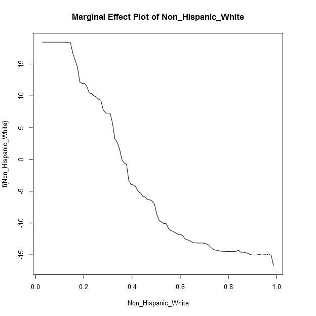
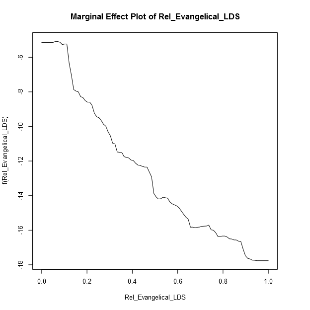
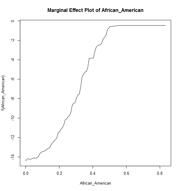
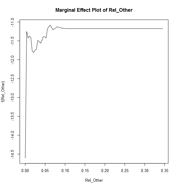
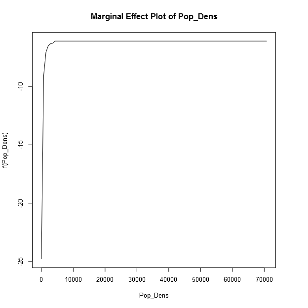
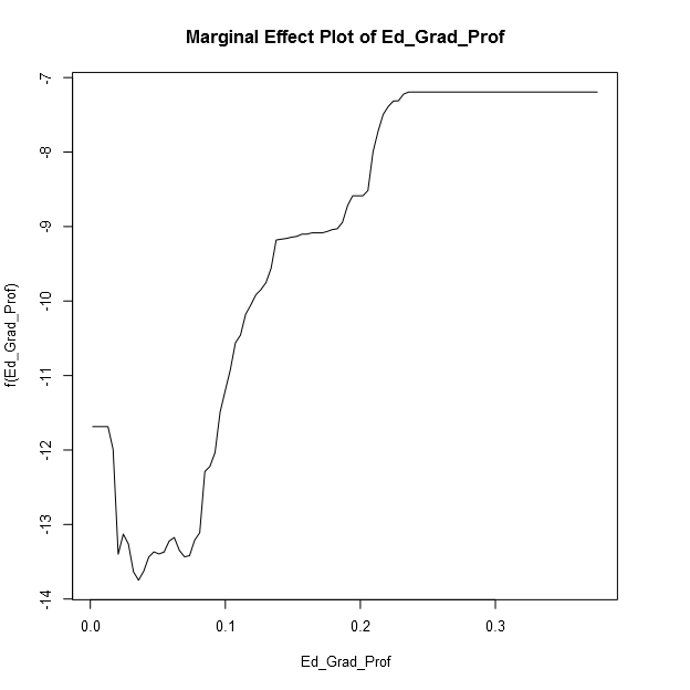
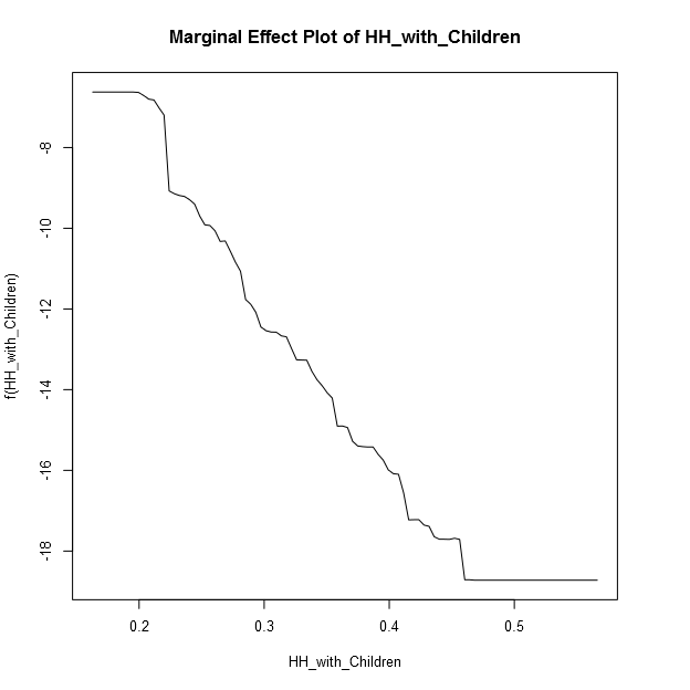
To assess the nature of the relationship between the predictor variables and county level PVI values, and see if it conforms to expectations, the marginal effects plots (also known as partial plots) are presented for the eight most important variables, in their order of importance. In the plots smaller (more negative) values indicate a stronger Republican lean, while larger (less negative or positive) values indicate a Democratic lean. The values on the y-axis are not that meaningful, it is really the shape of the plot (for numeric predictors) that matters.
The marginal effects plot for regions indicates that by far the most Republican leaning counties are located in Gulf Coast states, while the "Highlands", Prairie, and South Coast states also tend to lean Republican. The most hospitable counties for Democrats are in New England and the North Central states, followed closely by the Pacific states.
Counties with a high percentage of non-Hispanic whites lean much more strongly Republican, which is as expected.
Consistent with what we saw earlier, counties where a high share of religious congregation members are Evangelical or LDS strongly lean toward the Republican Party.
Counties with a high percentage of their population that is African American strongly lean toward the Democratic Party.
The higher the percentage of religious congregation members that are in the "other" (largely non-Christian) religion category, the more Democratic a county leans.
A county is likely to become more Democratic as its population density increases. However, there is a strong threshold effect in place in which the propensity to be Democratic leaning rapidly increases, but then abruptly reaches a plateau at around 7500 people per square mile.
Except when there is a very low percentage of adults 25 and older with a graduate or professional degree, as the percentage of this group increases, the more strongly a county is likely to lean toward the Democratic Party. The marginal effects plot (not included here) for the percentage of adults 25 or older who have a high school degree or equivalent indicates the opposite effect, with the propensity that a county leans Republican increasing with increases in the size of this educational attainment group.
As the percentage of households with children present increases, the more likely a county is to lean Republican. This suggests that the symbolic predisposition aspects of this variable are more important than its economic self-interest aspects.
Overall, the effects are very consistent with what we would expect, and with our earlier comparison of the most Republican and Democratic leaning counties. This analysis results in some additions to the descriptions of the "typical" highly Republican county or highly Democratic county. Specifically, a "typical" highly Republican county will be located in a rural area of a Gulf Coast, Prairie, "Highlands", or South Coast state; have a population that has a high percentage that is non-Hispanic white; have a high share of Evangelicals or LDS members among the population that are members of religious congregations; have an adult population age 25 and older that has an educational attainment level of a high school degree or its equivalent; and have a high percentage of households in which children are present. In contrast, a "typical" highly Democratic county is likely to be located in an urban area of a New England, North Central, or Pacific state; have a population that has a low percentage of non-Hispanic whites and a high percentage of African Americans; have a low share of Evangelicals or LDS members, but a high share of members of non-Christian faiths, among the population that belongs to a religious congregation; have an adult population age 25 and older who have earned an advanced degree; and have a low percentage of households in which children are present.
Access to the Alteryx Workflows and Data
After my last post, @dataMack provided a comment asking about obtaining access to the Alteryx workflows and data used in this series of blog posts. Two of the data sources in this analysis, the county level election returns and the 2012 county level demographic and socioeconomic data, are licensed data sources which we cannot publicly release. Surprisingly, historical county level election returns are not readily available (as discussed in this article on the FiveThrityEight website), and we have licensed this data from Dave Leip's Atlas of U.S. Presidential Elections. The demographic and socioeconomic data are from the 2012 estimates in the Experian CAPE data bundle that can be obtained as part of the Alteryx with Data licensing option. We are happy to provide anyone with the Alteryx workflows and unlicensed data used in this analysis, but, unfortunately, we cannot provide the licensed data.
What's Next?
This post is the fourth in a series of posts we are doing around the upcoming 2016 general election. The "main event" is the Alteryx 2016 Election app, to be released in early October. Between now and then there will be additional posts. The next two posts will be on "fundamentals" models for predicting election outcomes, where we will present one we have developed for voting at the county level.
1How the PVI we use is constructed is discussed in my first post on the 2016 election.
2Alaska only reports election results at the state level, so it is omitted from this analysis.

Chief Scientist
Dr. Dan Putler is the Chief Scientist at Alteryx, where he is responsible for developing and implementing the product road map for predictive analytics. He has over 30 years of experience in developing predictive analytics models for companies and organizations that cover a large number of industry verticals, ranging from the performing arts to B2B financial services. He is co-author of the book, “Customer and Business Analytics: Applied Data Mining for Business Decision Making Using R”, which is published by Chapman and Hall/CRC Press. Prior to joining Alteryx, Dan was a professor of marketing and marketing research at the University of British Columbia's Sauder School of Business and Purdue University’s Krannert School of Management.
Dr. Dan Putler is the Chief Scientist at Alteryx, where he is responsible for developing and implementing the product road map for predictive analytics. He has over 30 years of experience in developing predictive analytics models for companies and organizations that cover a large number of industry verticals, ranging from the performing arts to B2B financial services. He is co-author of the book, “Customer and Business Analytics: Applied Data Mining for Business Decision Making Using R”, which is published by Chapman and Hall/CRC Press. Prior to joining Alteryx, Dan was a professor of marketing and marketing research at the University of British Columbia's Sauder School of Business and Purdue University’s Krannert School of Management.
You must be a registered user to add a comment. If you've already registered, sign in. Otherwise, register and sign in.
